Prediction Model based on Moving Pattern

(1)

Prediction Model based on Moving Pattern

Zhengguang Xu , Member, IEEE

University of Science and Technology Beijing, Beijing, CHINA Email: [email protected]

Jinxia Wu and Shoude Qu

University of Science and Technology Beijing, Beijing, CHINA Email: {[email protected], [email protected]}

Abstract—For sintering process, based on the actual run status data, a new dynamics description method based on moving pattern is presented by constructing pattern moving space and defining moving variable in it. The moving variable is called as pattern class variable. And the prediction model is constructed based on pattern class variable. The feature vectors for constructing pattern moving space are extracted from the actual run status data by using partial least squares regression analysis method to cope with multicollinearity problem. Some simulations are given to verify the feasibility.

Index Terms—prediction model, moving pattern, pattern moving space, pattern class variable

I. INTRODUCTION

The sintering process is a preprocess for blast-furnace materials. A diagrammatic representation of the sintering plant is given in Fig.1. The raw materials are mixed together and are charged onto a moving strand (sinter car) to form a sinter bed. When the sinter cars pass under the ignition hood, the fuel in the surface of the bed is ignited. As sinter cars move forward, combustion is promoted by air drawn through the sinter bed into a series of wind boxes under the sinter bed. As the combustion zone moves further down the sinter bed and reaches the bottom, the sintering process is completed. The position on the strand where the combustion just progresses down to the bottom is the so-called burn-through point (BTP).

The sintering process is extremely complex. The mechanism of movement can not still be known completely. Where intertwines a series of physical and chemical changes such as heat transfer and mass transfer, combustion thermodynamics and chemical reaction kinetics, phase transition and moving boundary problems, hydrodynamics and pneumatics etc. It is difficult to describe the dynamics by equations of mathematical physics. Additionally, there are too many parameters for describing working conditions and product quality. It is difficult even impossible to determine degree of freedom

of working conditions. The dynamics of distribution, non-linearity, time variation and parameter perturbation can not be described accurately. Moreover, some physical processes such as particle granularity and its fluidity obey statistical laws in essence. The relationship between working conditions and product quality can not be represented by deterministic mathematical equations. There is only statistical correspondence relation between them.

1-sinter car 2-bedding material 3-mix feeding 4- ignition hood 5-bottom material 6-sintered material 7-cooling and wet zone 8-drying and preheating zone 9-combusion zone 10-sinter fusion and cooling zone 11-machine tail bend 12-wind box 13-star-shaped wheel 14-waste gas channel

Figure 1. A systematic diagram of sintering plant

Just the statistical characteristic makes this complex production process system different from the general complex system. It could be called as non-Newtonian mechanical system [1]. For this complex production process system, there is lack of effective dynamics description methods. We try to give a new method to describe the movement law obeying statistics by moving pattern.

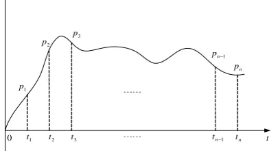
As is well known, the movement of system could be simply illustrated in Fig2.

L L

L L 1

t t2 t3 tn−1 tn

1

p

2

p 3

p

1 −

n

p

n

p F

t

0

Figure 2. Schematic diagram of movement trajectory Moving direction

Sinter

To suction

Manuscript received January 21, 2012; revised April 17, 2012; accepted April 23, 2012.

(2)

At each point in time t₁,t₂,t₃,_L,t_n₋₁,t_n , there corresponds different run statusP1,P2,L,P_n. It can be described by time-domain variables such as state variable, output variable, etc. while at each point in time

n n t

t t t

t₁, ₂, ₃,_L, ₋₁, , the run status also corresponds to a pattern. As time goes on fromt₁tot₂till tot_n, the run status of system will change from pattern 1 to pattern 2 till to pattern n under the inherent movement law of production process. Here pattern is a moving variable. Obviously, the movement law of system can also be described by the moving of pattern. The dynamics of system can be reflected by the variation of pattern class to which pattern belongs in different time.

In fact, early in 60's, pattern recognition developing in its initial stage has been used to solve control problems [2]. Later G. N. Saridis [3] presented a survey to state the applications of pattern recognition methods to control systems. More recent work on using pattern recognition for process control includes: structure identification of nonlinear system or distributed parameters system, state estimation, adaptive control etc [4]-[13]. when the dynamics of the system under control is not known. Sometimes it is only required to determine the class of the dynamics rather than its exact identification for making control decisions. In these methods, Pattern recognition is mainly used to solve system model identification or system state estimation problems. After that, the design of control law is still based on the time-domain model. In these methods pattern is not considered as a moving variable.

In this paper, different from traditional pattern-based control methods, the idea of moving pattern is proposed. That is we attempt to describe the dynamics of sintering process by the moving law of working condition pattern. The variable representing the moving of pattern is defined as pattern class variable. The dynamic behavior of the system is described by pattern class variable instead of state variable, output variable etc.

This moving pattern modeling method is composed of three parts, namely, construct “pattern moving space”, define pattern class variable, construct prediction model. First, based on the actual running status data, pattern classes are obtained by a clustering algorithm and these classes are used as the space scale to form “pattern moving space”. Then a variable which we called pattern class variable is defined in this “pattern moving space”. The value of this variable at any time represents a class since the space scale is pattern classes, so it has statistical characteristic. At last, prediction model is constructed in this pattern moving space based on pattern class variable by using time series analysis.

The outline of this paper is as follows. The next section presents the dynamics description method based on moving pattern including construct “pattern moving space”, define pattern class variable and construct prediction model. Section III gives simulations based on the sintering process data to illustrate the feasibility of this method. Finally, conclusions are drawn in section IV.

II. DYNAMICS DESCRIPTION METHOD BASED ON MOVING

PATTERN

A. Pattern Moving Space

Based on the actual run status data collected from sintering process of Jinan iron and steel plant, a method of statistical space mapping is given to construct “pattern moving space”. The main idea of this method is clustering in quality space and classifying in feature space, and a statistical mapping relation between these two spaces is built by using regress analysis method. The results of clustering in quality space are being mapped to feature space for forming pattern moving space.

Constructing feature space

Feature space of sintering process is constructed by image feature and measurement data. The image feature is extracted from the infrared image of sintering machine tail section including geometric characteristic of the image such as mean, variance, position distribution, etc. The measurement data include temperature and pressure of wind boxes. And the image feature together with the measurement data composes run status data set of sintering process. Feature vectors are extracted from the run status data set by using partial least squares regression analysis method to cope with multicollinearity problem. All these feature vectors span the feature space of sintering process.

Clustering in quality space

Quality space is constructed by the vectors of sinter quality indices, such as ferrous oxide (FeO), tumbler index (TI) and so on. To meet the need of distinguishability for product quality, the ISODATA clustering algorithm is chosen and improved. ISODATA algorithm is one of the most popular and well known clustering algorithms [16]. It can be viewed as a special case of the generalized hard clustering algorithmic scheme when point representatives are used and the squared Euclidean distance is adopted to measure the dissimilarity between vectors and cluster representatives. The splitting of pattern class in the algorithm is kept and the merging is canceled in keeping with the requirements of the service. After clustering in quality space, the pattern classes and classification rules are obtained.

Statistical space mapping

In order to establish the statistical mapping relation between feature space and quality space, the regress analysis method is used. FeO and TI are selected as dependent variables. And the feature vectors extracted from the actual run status data set of sintering process are as independent variables. The statistical mapping relation between these two spaces is established as follows:

) ( )

( )

(

) ( )

( )

(

, 2 2

2 , 2 1 1 , 2 0 , 2 2

, 1 2

2 , 1 1 1 , 1 0 , 1 1

t x b t x b t x b b t y

i i

i i + +

+ =

+ +

+ =

L L

(1)

Where

y

₁

(

t

)

and y2(t) are quality indices in quality space, xi(t)is feature vectors in feature space.

(3)

space can be mapped to feature space. And those classes in feature space are as the space scale to form “pattern moving space”.

If the data is collected in a long enough period of time, the “pattern moving space” constructed based on these actual run status data can be considered as the run subspace of the system. Dynamics description and control problems can be discussed in this space. When the actual run status sample is out of the” pattern moving space”, the “pattern moving space” can be expanded by using the following method.

When a new pattern sample is classified to its class, the distance between the pattern sample and this class center is calculated. If this distance is more than the class radius, then the new class generates. The new class center is just the pattern sample and the new class radius is the distance minus the class radius.

The above algorithm of constructing pattern moving space is summarized as follows:

Step 1: Constructing feature space and quality space. Based on the actual run status data, the feature space is constructed by using the partial least squares algorithm to extract feature vectors.

According to the needs of the actual production process, FeO and TI are chosen for forming the quality space.

Step 2: Establishing the statistical mapping relation between feature space and quality space by using regress analysis method as shown in equation (1).

Step 3: Clustering in quality space by using the improved ISODATA clustering algorithm. The class center Zj(Jy) , the class radius Dmax,j,y and the classification rule D(yk,Zj(Jy))can be obtained.

Where

y

_k is the pattern sample in quality space,

c

is the number of class, ω_jis the jth class,

. , , 2 , 1 }, , , 2 , 1 )), ( , ( max{ ,

max, D y Z J k n j c

D jy= ω_j k j y = L = L

} , , 2 , 1 )), ( , ( min{ )) ( ,

(y Z J D y Z J j c

D _k _j _y = _k _j _y = _L

Step 4: Statistical space mapping.

Using the statistical mapping relation equation (1), the clustering results in quality space are mapped to feature space for forming pattern moving space scale. In the feature space, the class center Zj(Jx) , the class

radius Dmax,_j,_x and the classification rules ))

( , (xk Zj Jx

D can also be obtained.

Where

x

_k is the pattern sample in feature space.

. 2 , 1 }, , , 2 , 1 )), ( , ( max{

,

max, D x Z J k n j c

D _j_x _k _j _x

j = L = L

= _ω

{

D x Z J j c

}

J

Z x

D( _k, _j( _x))=min ( _k, _j( _x)), =1,2,_L, Step 5: Expanding pattern moving space.

For every new pattern sample x_k,k=1,2_L,n , the distanceD(x_k,Z_j(J_x)) between the new pattern sample

and its class center can be calculated. If D(x_k,Z_j(J_x))>D_max,_j_,_x , then the subspace is expanded by creating a new class c=c+1. The new

class center is the new pattern sample and the new class radius isDmax,_j+1,_x =D(x_k,Z_j(J_x))−Dmax,_j,_x.

Detail algorithm can be seen in reference Z.G.Xu [14-15].

B. Pattern Class Variable

In order to describe the movement of system in pattern moving space, a variable called pattern class variable is defined.

Assuming that

{

sx(k)

}

and

{

mx(k)

}

denotes measurement sample series and pattern sample series, respectively. A variable

dx

(

k

)

that satisfy the following transform is defined as pattern class variable.

mx

(

k

)

=

T

(

sx

(

k

))

(2)

dx

(

k

)

=

F

(

mx

(

k

))

(3)

Where T(⋅) and F(⋅) are feature extraction and classification, respectively.

Obviously, pattern class variable has two main characteristics:

(i) It is a variable over time. (ii) It has the class attribute.

Since pattern class variable denotes a pattern class, it has statistical characteristic. So the dynamics description method based on pattern class variable can well reflect the statistical characteristics of the plant. It is different from the existing statistical modeling methods. But pattern has not calculation property, that is to say pattern1+pattern2

≠

pattern 3. In order to calculate, the first principal component of the corresponding pattern class is taken as pattern class variable’s measurement value after classification. Pattern class variable is used to describe the dynamics of the system by the change of pattern class over time in “pattern moving space”.

C. Prediction Model based on Pattern Class Variable Prediction Model

The system prediction model can be built as

)))

(

)

2 (

),

1 (

(

))

(

ˆ~

(

)

(

ˆ

p

k

dx

k

dx

k

dx

f

F

k

x

d

F

k

x

d

−

=

L

(4)

Where

dx

(

k

)

is pattern class variable, F(⋅)denotes

classification,

d

x

ˆ~

(

k

)

is the initial prediction output of

pattern class variable and dxˆ~(t)= f(⋅) is the initial prediction model.

d

x

ˆ

(

k

)

denotes the final prediction output of pattern class variable in “pattern moving space”. This is a prediction process including two steps. The

first step is to obtain the initial prediction output

d

x

ˆ~

(

k

)

(4)

)

(

)

(

)

2 (

)

1 (

)

(

ˆ~

2 1

k

p

k

dx

k

dx

k

dx

k

x

d

p

α

ϕ

+

−

+

−

+

−

=

_L

(5)

The second step is to obtain the final output of pattern class variabledxˆ(k)by classifying the initial prediction output

d

x

ˆ~

(

k

)

, that is

d

x

ˆ

(

k

)

=

F

(

d

x

ˆ~

(

k

))

.

Prediction Algorithm

Because the pattern class variabledx(k) is obtained by classifying the pattern sample series or initial prediction

outputdxˆ~(k), the effect of the random error or random disturbance has been overcome effectively in the pattern classification process. Based on the prediction model (4) and the initial prediction model (5), the multi-step ahead prediction algorithm in pattern moving space is given as follows: )) 1 ( ˆ~ ( ) 1 ( ˆ ) 1 ( ) 1 ( ) ( ) 1 ( ˆ~ ,

1 ₁ ₂

+ = + + − + + − + = + = k x d F k x d p k dx k dx k dx k x d m p

ϕ

L (6) )) 2 ( ˆ~ ( ) 2 ( ˆ ) 2 ( ) ( ) 1 ( ˆ ) 2 ( ˆ~ ,

2 ₁ ₂

+ = + + − + + + + = + = k x d F k x d p k dx k dx k x d k x d m p

ϕ

L (7)

M

))

(

ˆ~

(

)

(

ˆ

)

(

)

1 (

)

(

ˆ

)

1 (

ˆ

)

2 (

ˆ

)

1 (

ˆ

)

(

ˆ~

,

1 1 2 1

m

k

x

d

F

m

k

x

d

p

m

k

dx

k

dx

k

x

d

k

x

d

m

k

x

d

m

k

x

d

m

k

x

d

p

m

p m m m

+

=

+

−

+

−

+

−

+

−

+

=

+

≤

+ −

ϕ

L

(8)

))

(

ˆ~

(

)

(

ˆ

)

(

ˆ

)

2 (

ˆ

)

1 (

ˆ

)

(

ˆ~

,

2 1

m

k

x

d

F

m

k

x

d

p

m

k

x

d

m

k

x

d

m

k

x

d

m

k

x

d

p

m

p

+

=

+

−

+

−

+

−

+

=

+

>

ϕ

L

(9)

WhereF(⋅)denotes classification.

Estimating the parameters of prediction model The pattern class variable

dx

(

k

)

can be obtained by classifying the pattern sample series, it also can be obtained by classifying the initial prediction

outputdxˆ~(k), so the parameters

ϕ

₁,

ϕ

₂_L

ϕ

_pof prediction model can be estimated according to the follow equation by using least squares method:

)

(

)

(

)

2 (

)

1 (

)

(

₁ ₂

k

p

k

dx

k

dx

k

dx

k

dx

p

α

ϕ

+

−

+

−

+

−

=

_L

(10)

ϕˆ=(DXTDX)−1DXTDY (11) Where

[

]

T

N k dx k dx k dx k dx

DY= ( ), ( +1), ( +2),_L, ( + ) (12)

⎥ ⎥ ⎥ ⎥ ⎦ ⎤ ⎢ ⎢ ⎢ ⎢ ⎣ ⎡ − + − + − + + − − − − − = ) ( ) 2 ( ) 1 ( ) 1 ( ) 1 ( ) ( ) ( ) 2 ( ) 1 ( p N k dx N k dx N k dx p k dx k dx k dx p k dx k dx k dx DX L M O M M L L (13)

Determining the order of prediction model

As the effect of the random error or random disturbance has been overcome effectively in the pattern classification process, the model residuals only depend on the choice of model order. So we can estimate the order of prediction model by judging

α

(

k

)

equals to zero or not.

α

(

k

)

=

dx

(

k

)

−

d

x

ˆ

(

k

)

(14)

Where dx(k) is the actual running status output obtained by classifying the pattern sample, dxˆ(k)is the final prediction output by classifying the initial prediction outputdxˆ~(k).

If the final prediction output

d

x

ˆ

(

k

)

equals to the actual pattern class variabledx(k), thenα(k)equals to zero. Otherwise it is not true. So the estimation steps of model order can be given as follows:

Step1 Calculate the estimation of pattern class variable

)

(

ˆ

t

x

d

according to (6-9).

Step2 Obtain the pattern class variable

dx

(

k

)

by classifying the pattern sample.

Step3 Calculate the residualsα(k)according to (14). Step4 If the residuals

α

(

k

)

≠

0

, increase the orderp= p+1, returning to step1.

If

α

(

k

)

=

0

, then the order P is regarded as the final order of the model.

Notes: in actual calculation process,

α

(k)may not equals to zero, for a given small enough constantε , when

α

(k)<

ε

, the order P is regarded as the final order of the model.

III. SIMULATION

(5)

class is taken as its value. It is shown in table 1. The before 40 pattern samples are used to estimate the parameters of prediction model (5) and the last 3 pattern samples are used to verify the effectiveness. Given the order of model

p

=

3 ,

4 ,

5 ,

6 ,

7

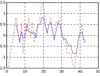
respectively, the parameters of each prediction model are estimated and shown in table 2. The results of initial prediction are shown in table 3-7. After classifying the initial prediction output, the final prediction output can be obtained. It is shown in figure 3-7. Where dotted red line denotes 43 sets of actual pattern class variable time series, solid blue line denotes the final prediction output series.

From all the results of prediction we can see that the model is capable of representing the process dynamics. But the relative error still exits. The computer calculation error and lacking of sample data may be the cause.

TABLE I.

PATTERN CLASS VARIABLE TIME SERIES

Sample 1 Sample 2 Sample 3 Sample 4 Sample 5 -1.434700 -0.848450 -2.416400 0.164120 0.809250 Sample 6 Sample 7 Sample 8 Sample 9 Sample 10 -0.848450 -0.315550 2.228500 -0.848450 -0.315550 Sample 11 Sample 12 Sample 13 Sample 14 Sample 15 0.164120 0.809250 -0.116400 1.418867 -0.315550 Sample 16 Sample 17 Sample 18 Sample 19 Sample 20 0.164120 0.495100 -0.315550 1.418867 1.418867 Sample 21 Sample 22 Sample 23 Sample 24 Sample 25 0.495100 0.164120 -1.434700 0.809250 0.164120 Sample 26 Sample 27 Sample 28 Sample 29 Sample 30 -0.198633 0.598900 0.598900 0.809250 0.080000 Sample 31 Sample 32 Sample 33 Sample 34 Sample 35 0.198633 -0.198633 -0.848450 -0.803600 -0.803600 Sample 36 Sample 37 Sample 38 Sample 39 Sample 40 2.300000 -1.434700 -0.848450 -0.198633 0.164120 Sample 41 Sample 42 Sample 43

0.495100 -0.315550 -0.315550

TABLE II.

THE INITIAL PREDICTION OUTPUT WHEN P=3 P=3: 0.502273 0.315560 -0.217645

P=4: 0.512082 0.295367 -0.240466 0.080151

P=5: 0.487030 0.294332 -0.234532 0.110626 0.045262 P=6: 0.499696 0.291062 -0.212582 0.079602 -0.020281

0.086650

P=7: 0.493458 0.329751 -0.209236 0.062385 -0.002438 0.078096 -0.068291

TABLE III.

THE INITIAL PREDICTION OUTPUT WHEN P=3 Sample 3 Sample 4 Sample 5

-0.113974 0.167519 0.526932

Sample 6 Sample 7 Sample 8 Sample 9 Sample 10 0.302080 -0.282832 0.165516 -0.168487 -0.097273 Sample 11 Sample 12 Sample 13 Sample 14 Sample 15 0.456083 0.327907 0.161182 0.087951 0.055830 Sample 16 Sample 17 Sample 18 Sample 19 Sample 20 -0.147489 0.369143 0.526978 0.860269 0.984267 Sample 21 Sample 22 Sample 23 Sample 24 Sample 25 0.387604 -0.070142 0.192709 0.526978 0.230044 Sample 26 Sample 27 Sample 28 Sample 29 Sample 30 -0.224107 0.202411 0.533032 0.465106 0.165201 Sample 31 Sample 32 Sample 33 Sample 34 Sample 35 -0.250652 -0.179860 -0.445603 -0.628132 -0.472550 Sample 36 Sample 37 Sample 38 Sample 39 Sample 40 -0.731639 -0.955939 -0.595949 -0.055250 0.204413 Sample 41 Sample 42 Sample 43

0.343696 -0.037978 -0.365823

TABLE IV.

THE INITIAL PREDICTION OUTPUT WHEN P=4 Sample 4 Sample 5

0.079871 0.470753

Sample 6 Sample 7 Sample 8 Sample 9 Sample 10 0.258311 -0.294555 0.238879 -0.168547 -0.113225 Sample 11 Sample 12 Sample 13 Sample 14 Sample 15 0.512964 0.250859 0.187956 0.090862 0.108160 Sample 16 Sample 17 Sample 18 Sample 19 Sample 20 -0.162505 0.425888 0.495881 0.859700 0.990747 Sample 21 Sample 22 Sample 23 Sample 24 Sample 25

0.396290 0.002812 0.296675 0.560855 0.217168 Sample 26 Sample 27 Sample 28 Sample 29 Sample 30 -0.208155 0.273413 0.544500 0.431361 0.183979 Sample 31 Sample 32 Sample 33 Sample 34 Sample 35 -0.224682 -0.114761 -0.438969 -0.630269 -0.460762 Sample 36 Sample 37 Sample 38 Sample 39 Sample 40 -0.777828 -0.989830 -0.610041 -0.111519 0.114405 Sample 41 Sample 42 Sample 43

0.281768 -0.070737 -0.360691

TABLE V.

THE INITIAL PREDICTION OUTPUT WHEN P=5 Sample 5

0.357644

0.177222 -0.106826 -0.353510

TABLE VI.

THE INITIAL PREDICTION OUTPUT WHEN P=6

(6)

TABLE VII.

THE INITIAL PREDICTION OUTPUT WHEN P=7

Sample 7 Sample 8 Sample 9 Sample 10 -0.228191 0.240522 -0.112531 -0.077651 Sample 11 Sample 12 Sample 13 Sample 14 Sample 15 0.451685 0.237897 0.282825 -0.010556 0.220930 Sample 16 Sample 17 Sample 18 Sample 19 Sample 20 -0.185695 0.454091 0.442751 0.929139 0.963645 Sample 21 Sample 22 Sample 23 Sample 24 Sample 25 0.498951 0.061369 0.309282 0.611222 0.267188 Sample 26 Sample 27 Sample 28 Sample 29 Sample 30 -0.240966 0.223977 0.570304 0.488105 0.176416 Sample 31 Sample 32 Sample 33 Sample 34 Sample 35 -0.231779 -0.070894 -0.433723 -0.625047 -0.544930 Sample 36 Sample 37 Sample 38 Sample 39 Sample 40 -0.811764 -1.018511 -0.720631 -0.161561 0.098800 Sample 41 Sample 42 Sample 43

0.243913 -0.060379 -0.320917

0 10 20 30 40 50

-1.5 -1 -0.5 0 0.5 1 1.5

Figure 3. The final prediction output when P=3

0 10 20 30 40 50

-1.5 -1 -0.5 0 0.5 1 1.5

0 10 20 30 40 50

-1.5 -1 -0.5 0 0.5 1 1.5

0 10 20 30 40 50

-1.5 -1 -0.5 0 0.5 1 1.5

0 10 20 30 40 50

-1.5 -1 -0.5 0 0.5 1 1.5

IV. CONCLUSION

In this paper, dynamics description for sintering process based on moving pattern has been proposed. The main advantage of this method can reflect the statistical characteristic of this system. But it is different from the autoregressive model (AR) though they have the same structure in the initial prediction model. There are two reasons to explain their differences. The first is that the prediction model is a two-step prediction model, it has a classification process. The second reason is that the variable has statistical characteristic. Pattern moving space is constructed by statistical space mapping method to meet the need of distinguishability for quality indices. A variable called pattern class variable is defined in this space and the prediction model based on pattern class variable has been built. At last, an example of the sintering production process is given to verify the research. The results have shown that the proposed method is feasible. Further research is focus on controller design based on moving pattern, and the relationship between the pattern moving space granularity and system regulation performance can also be studied.

ACKNOWLEDGMENT

(7)

REFERENCES

[1] S.D.Qu, Z.F.Li ,and S.M.Zhou. “Pattern recognition and

intelligent automation (Translation Published Conference

Proceedings style, Chinese)”. Proc. of intelligent

automation in China. 1995, pp.64-66.

[2] B.Widrow and F.W.Smith, Pattern recognition control

systems, in computer and Information Sciences, Washing,

DC.Spartan, 1964.

[3] G.N.Saridis, Application of pattern recognition method to

control systems, IEEE Trans.Automatic Control, 1981.

26(3). 638-645.

[4] E.H.Bristol, Pattern Recognition: an Alternative to

Parameter Identification in Adaptive Control, Automatic,

1977. 13(2). 197-202.

[5] GEORGE N. SARIDIS and ROBERT F. HOFSTADTER,

A Pattern Recognition Approach to the Classification on

Nonlinear Systems, IEEE Trans on SMC, 1974;4;362-371.

[6] M.Cadaparthi B.Brahmanandam, Member, IEEE, and B. N.

Chatterji, A pattern recognition approach to model

characterization of distributed systems, IEEE Trans.SMC,

1987,17(3).488-495.

[7] Ye N. and Lu Y.Z. An Application of Pattern Recognition

to System Modelling, Proc.of 8th IFAC Symposium on

Identification and System Parameter Estimation, 1988, pp. 1702-1707.

[8] Kar-Ann Toh and R. Devanathan, Pattern-Based

Identification for Process Control Applications, IEEE

Trans. Control Systems Technology, 1996.4(6).641-648.

[9] Huaglory Tianfield, Online-Data-Based Pattern

Recognition of Transient Responses and Suboptimal

Iteration of Control Parameters. IEEE Trans.Control

Systems Technology, 2000. 8(3). 532-544.

[10]Daniel Sbarbaro and Tor A. Johansen, Analysis of

Artificial Neural Networks for Pattern-Based Adaptive

Control. IEEE Trans. Neural Networks,

2006.17(5).1184-1193.

[11]Pregelj Boštjan, Strmcnik, Stanko and Gerkšic, Samo,

Pattern recognition-based supervision of indirect

adaptation for better disturbance handling, ISA

Transactions, 2007.46(4).561-568.

[12]C. Wang and D.J. Hill. Deterministic learning and rapid

dynamical pattern recognition, IEEE Transactions on

Neural Networks, 2007,v.18, pp. 617-630.

[13]Rachelle Howard and Douglas Cooper. A novel

pattern-based approach for diagnostic controller performance

monitoring, Control Engineering Practice 18, 2010, pp.

279-288.

[14]Z.G.Xu, H.T.Wang andS.D.Qu A pattern recognition

method based on statistical space mapping, Journal of

University of Science and Technology Beijing, 2001.23(2). pp. 181-183.

[15] Z.G.Xu, S.D.Qu and L.R.Yu. “Self-learning pattern

recognition method based on the statistical space mapping

(Translation Journals style, Chinese)”, Journal of

University of Science and Technology Beijing, China, 2003.25(5). pp. 480-482.

[16]Anderberg M.R., “Cluster analysis for applications”,

Academic press, 1973.

Zhengguang Xu received the PhD degree (2000) in control science and engineering from University of Science and Technology Beijing, Beijing, CHINA. He is now a professor at University of Science and Technology Beijing. His current research interests include non-Newtonian mechanical system control, pattern recognition, image processing, Petri nets.

Jinxia Wu received the MSc degree (2007) in mathematics from Bohai University, CHINA. She is now a PhD candidate at University of Science and Technology Beijing. Her current research interests include non-Newtonian mechanical system control, pattern recognition, Petri nets.