Efficient Localization Technique for Complex Anchor Distribution in WSN

Efficient Localization Technique for Complex

Anchor Distribution in WSN

Soumya Simpi

, P.N.Simpi

, Kavya Simpi

Assistant Professor, Dept. Of ECE, KLEIT, Hubballi, India #2

Lecturer, BVVS Polytechnic, Bagalkot, India #3

Student, Dept. of EI, BEC Bagalkot, India

Abstract

WSN is a very fast growing technology in recent days. Localization is a very critical and important issue. In many applications of WSN like target tracking, health monitoring, military and environmental monitoring the data is of very important. So without the knowledge of the location the data is of no use in WSN. Hence localization needs to be done in a proper way.

Many proposed localization algorithms are concentrated on improving the localization accuracy without considering the efficiency. But in this proposed work it is showed that the proposed scheme of modified DV-Hop localization algorithm achieves good accuracy and less convergence time for the networks by using the median hop value. The simulation results showed the minimum localization error, less execution time and minimum amount of energy consumption. The scheme works fine with complex anchor distributions and also compared with improved DV-Hop algorithm.

Keywords - DV-Hop, sensor node

I. INTRODUCTION

With the development in technology many sensor techniques, low powered electronic technique, radio technique and inexpensive wireless sensor networks (WSN’s) came into picture. Then wireless sensor networks have come. WSN consists of large number of sensor nodes typically around hundreds to thousands of nodes. Fig 1.1.shows number of sensor nodes is sending information to the sink node via the target. WSN can be used in most of the applications like in industry, home automation, military, environmental monitoring, smart structure, medical applications and in many others.

In many WSN applications the information is of no use if the location is unknown. Location information is also required for services like location aware services, coverage area management, disaster event notifications, geographic in addition to context based routing protocols, target tracking, rescue and coverage.

Fig 1.1: Wireless Sensor Network

Localization is in generally locating the node in a fixed position. The localization is the process of finding the position of nodes based on the input data. Simple localization of sensor nodes and anchor nodes (beacon nodes) are shown in fig 1.2. Anchor nodes are the nodes present in the network where the position of the nodes is previously known. These nodes may be equipped with GPS (Global Positioning System). In the figure the nodes marked with shaded circles are the anchor nodes and the nodes represented with hollow circles are the simple sensor nodes for which the location needs to known.

Fig 1.2: A simple network with sensor and anchor nodes

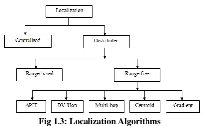
There are many localization algorithms that have been proposed as following.

The classification of the algorithm is explained in the previous survey paper [2].

II. LITERATURE SURVEY

[1]In this paper the author proposes the application of WSN used in environmental monitoring. He used an IRIS mote hardware platform that collects seven environmental parameters and the system also made a number of achievements. He also utilized more number of nodes to provide long-term environmental monitoring. In his future work the data network security is also considered. [2]In this paper, the author has classified many

localization algorithms. The author considered DV-Hop algorithm and also considered anchor distributions.

[3]In this paper the author has considered WSN as growing technology and determination of location of nodes is one of the important task. So author analyzed various localization techniques and distinguished between range based and range free localization algorithms. Localization algorithm for mobility of anchor nodes, proposing a localization technique for the combined mobile and static nodes and scaling the existing algorithms is considered in the future work.

[4]In this paper, author has discussed the difficulty in placing the nodes that is localization. He explained the different localization methods and also range based and range free techniques. Author has considered localization the important issue in WSN as nodes do the collection of data.

[5]In this paper, the author discussed different range

free localization algorithms and he compared the performance. So author has presented different localization algorithms and for complex anchors he worked on existing algorithms.

In this paper, author presented an improved DV-Hop that improves the original DV-DV-Hop algorithm. Anchor nodes importance is explored in the DV-hop algorithm. Author showed that the quantity of anchor nodes could influence the localization average error and location coverage of the algorithm. Higher location coverage can be obtained by lower location error.

[7]In this paper, the author proposed localization scheme called as DV-max Hop that can achieve good efficiency and precision. Authors formulated the multi-objective optimization functions they are the number of transmission in localization phase as well as to minimize location errors and estimate the performance of design using extensive simulation on several anisotropic and isotropic topologies. The proposed DV-Hop algorithm scheme can achieve dual objective of efficiency and accuracy for various scenarios. The lately proposed algorithms are persistent on localization exactness without considering efficiency in terms of energy and communication

cost. The simulation results uses extended simulation framework.

[8]In this paper, the author compared the analysis of range free algorithms of both DV-Hop and Centroid algorithm. Simulation results showed that DV-Hop algorithm provides better accuracy than Centroid algorithm in finding the unknown nodes in wireless sensor network.

In literature survey number of localization algorithms are studied. It is understood that improved DV-Hop algorithm is better compared to other algorithms. There are different algorithms in range based and range free algorithms. DV-Hop algorithm is in the category of range free technique. In DV-Hop algorithm the parameter MaxHop is considered in broadcasting. To overcome the problem that is in DV-Hop, it sends only packets without any identification in that packet improved DV-Hop algorithm is introduced. But in modified DV-Hop enhancement improved over DV-Hop is done in the present work. In this present algorithm median hop is taken for the broadcasting which is explained in next sections.

III. PROPOSED METHODOLOGY

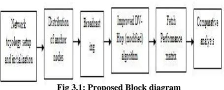
In literature survey many localization algorithms are studied. Range based and range free methods are the part of localization algorithms. In the study matlab software is used. DV-Hop algorithm achieves better accuracy for anisotropic networks. The proposed block diagram is shown below in fig 3.1.

A. Block Diagram

Fig 3.1: Proposed Block diagram

Initially according to the block diagram network topology setup like are, number of nodes and initialization is done. After generating the network topology distribute the anchor nodes in the network. Then these anchor nodes starts broadcasting. Modify the DV-Hop algorithm. After this fetch

the performance matrix of the network and then finally do the comparative analysis.

B. Network Model:

Describing the network model and parameters used in the proposed scheme.

N = Total number of nodes in the network Na = Number of anchor

nodes

Nr = Number of regular nodes

A_r = Anchor ratio (N_a/N) Aid = Anchor node ID

Nd = Network density

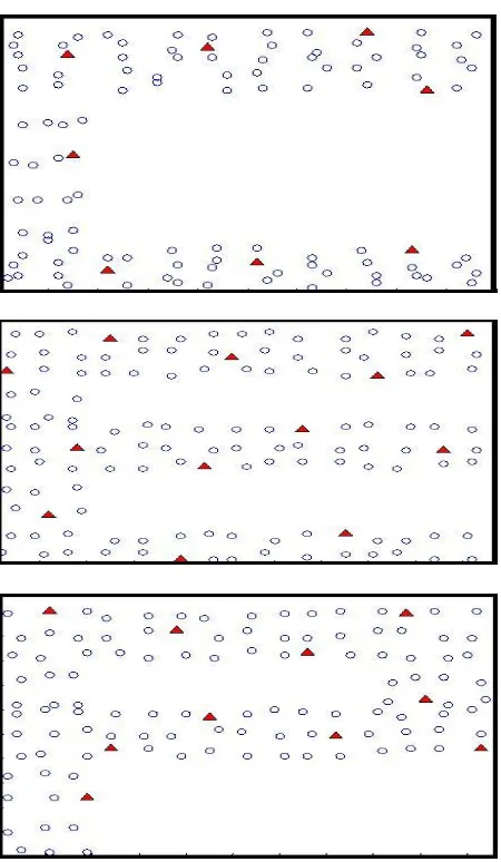
For the purpose of study two dimensional (2D) square area is considered for wireless node deployment. Consider C, E and P shape network as shown in below fig 3.2

Fig 3.2 : Node deployment in (a) C-shape (b) E-shape (c) P-shape

Based on the square area of deployment number of nodes are considered. In this case it is assumed that all nodes have the same transmission range (R). Every node in the network is able to communicate with all of its neighbours such that they must be within the range R. Anchor nodes position is previously known with the help of GPS. As shown in the fig 3.2. the anchor nodes are in triangle shape and sensor nodes are in circle shape

C. Anchor Distribution Strategies:

Accuracy and efficiency of the localization algorithm is dependent on the anchor distribution strategies. It is assumed that anchor nodes and other nodes in the network are randomly as well as uniformly distributed [7]. It is necessary that anchor nodes must be placed at the right places in the

network. Some anchor distribution methods are as following [7].

Random

In this method anchor nodes are deployed randomly. Localization errors are possible if a number of the regular nodes are unable to get the distance estimation from the at least three anchors. In some cases nodes may remain unlocalized. The random strategy works fine when anchor ratio is high or in a densed network.



 Grid: 

In this method of anchor distribution, anchors are uniformly placed and cover the whole network. Let us start from one end of the network say bottom left and then select the anchor nodes as Xth place node. Anchor ratio is X (Ar). Consider for example

for 100 nodes in the network if the desired anchor ratio (Ar) is 10% then the value of X will be 10

(100/10) , such that the 10th node will be the anchor node. We can use this for simulation but uniform anchor distribution is the network shape and uniformity of sensors depends on the uniform anchor distribution.



 Cluster Centroid

The nodes exact or approximate locations are known or can be calculated in some network deployment schemes. In such cases clustering algorithm can be utilized to find the distribution of anchors. Based on the desired anchor ratio (Ar) the

number of required clusters can be determined. It utilizes expectation maximization (EM) algorithm and it is studied in detail [7].



D. Modified DV-Hop algorithm



The DV-Hop algorithm is explained in [6]. The modified DV-Hop is explained in three steps.

 Step 1: Initially before broadcasting a message the hop-count value is initialized to one. The beacon message containing the anchors location with the initial hop-count value is broadcasted by each anchor node in the network. The anchor node broadcasting and coverage area for the network shapes C, E and P. After receiving a beacon message by each node, it maintains a minimum hop-count value per each anchor node.

For particular anchor node the higher hop-count value with a beacon message is considered as stale information and this message will be ignored. Then the beacon message that is not stale is flooded to the entire network with the hop-count value and will be incremented at every intermediary hop. So with this mentioned method the minimal hop-count value will be send by every anchor node and all nodes in the network get the information.

including a median value of hop-size and identifier Id. After getting this package the information is added to the table and it broadcasts to its neighbor nodes. The HopSizei is

calculated by the anchor nodes. It is in the step 1 of the DV-Hop algorithm. After broadcasting in step 1 all of nodes gets HopSizei.



 Step 3: As stated in step 3 of the DV-Hop algorithm based on the hop length and hops to the beacon nodes distance to

beacon nodes is calculated by using the formula [6].

di = hops X HopSizei 3.1



Let (Xi , Yi ) be the known location of the

anchor node i and (x , y) be the source node location and di is the distance between the ith

anchor node and unknown node. It is given by the below formula.

di = sqrt((Xi – x) 2

+ (Yi –y ) 2

)

From the above equation 3.7 we get the following [6].

Xi2 + Yi2 – 2Xix – 2Yiy + x2 + y2 = di2

di2 – Ei = 2Xix – 2Yiy +K

where Ei = Xi2 + Yi2 K = x2 + y2

Let

Zc = [x, y, K]T

−2𝑋1 − 2𝑌2 1

−2𝑋2 −2𝑌2 1

Gc= :

:

−2𝑋i −2𝑌i 1

And

𝑑

−

𝐸

𝑑

−

𝐸

ℎ 𝑐

= :

:

𝑑

−

𝐸

So we have Gc Zc = hc

From the above equation 3.12 we have

𝑍𝑐 = (𝐺cT𝐺c)𝐺cTℎc

Equation 3.8 is found by the least square (LS) algorithm [20]. So the unknown node (x, y) coordinated are given by

𝑥 = 𝑍𝑐 (1)

𝑦 = 𝑍𝑐 (1)

(a)

(b)

Fig 3.3: The modified DV-Hop for C-shape (a)Localization ccuracy (b)Average Hop Vs Number of packets

The modified DV-Hop algorithm is simulated for C, E, P shapes. Considering the simulation parameters the graphs are plotted for those shapes as shown in figures 3.3, 3.4, 3.5.

(a)

3.7

3.2

3.3

3.5

3.4

3.6

3.8

Fig 3.4: The modified DV-Hop for E-shape (a)Localization Accuracy (b)Average Hop Vs Number of packets

Fig 3.5: The modified DV-Hop for P-shape (a)Localization Accuracy(b)Average Hop Vs Number of packets

E. Flow Chart:

Flowchart for the modified DV-Hop algorithm is as shown in the fig 3.6. Initially the network topology setup and initialization is done. Anchor node distribution is also done in random, grid or cluster Centroid method. After this, broadcasting of package to the nodes is done. Then this package is broadcasted to all of its neighbours.

And then nodesreceive the package containing node Id

and hop-sizei with the initial hop-count value 1 is

broadcasted. Then the hop-count value increases for

every intermediate step. Then the median Hop-Sizei

value is taken instead of average hop-seize in the improved DV-Hop algorithm. After this the distance is calculated. Then the unknown nodes get its location and the process is continued till all the unknown nodes compute their location.

Fig 3.6: Flow Chart

IV. SIMULATION

The proposed scheme is simulated using matlab. Matlab is developed by math works and is a programming language. It is also a fourth generation programming language. This software is used because it allows plotting of data and functions, creation of user interfaces, manipulations of matrix, and it interfaces the programs that are written in other languages including C, C++, C#, Java and Python.

section and the algorithm is compared with the previously proposed algorithms to get the results.

A. Simulation Setup:

In the proposed scheme for simulation matlab is used. For C, E, P shapes different codes are written. For all of these shapes 100X100 area is considered. Total number of nodes are 100 and 30 are the number of anchor nodes. Communication range of each node in all shapes of the network is 15m, radius is 15m and anchor ratio (Ar) is set typically around 6-9%.

In node deployment schemes number of nodes are deployed in a given two dimensional (2D) area. Consider the nodes in a circular shape and anchor nodes in a triangle shape. Some parameter values are noted before the simulation and also after the simulation. Localization accuracy depends on the anchor ratio. Hence we get the good results with the above mentioned anchor ratio.

B. Simulation Parameters:

Some of the performance matrices for simulation considered for simulation are anchor ratio, localization error, algorithm runtime, number of packets per node, average hop and energy consumed.

1. Localization error

Localization error is the distancebetween the estimated and the actual node position.

Error = √((xactual – xestimated)2 + ( yactual – estimated)2 )

Based on the location error the performance of the network is evaluated.

2. Anchor ratio

Anchor ratio determines the requirednumber of clusters. It can be defined as the ratio of number of anchor nodes to the total number of nodes in the network. Anchor ratio for the network should be minimum. If the anchor ratio is less then localization accuracy will be more.



3. Algorithm runtime

It can also be called as convergence time. It is measured in milliseconds (msec). It is one of the

important performance measure of the algorithm. Time should be less to get the best estimation. (Note: The time depends on the processor speed and background works.)

4. Energy consumption

Energy consumption is one of the important parameter in WSN. The battery supplies power to all nodes in the network. The nodes in the network must consume minimum amount of energy. The total energy consumption is the energy consumed by the complete network. It is proportional to the packet size and communication cost. The total energy consumed by the network is calculated using the below formula

E = Esense X Dsense + Etx X Dtx

The energy can be the sum of different componentsand these are determined by the duty cycle. Esense is the energy consumed by the node for

every sensing and Dsense is duty cycle for sensing. The

subscript tx refers to the send component.

5. Number of packets per node

It is defined as the number of packets considered per node in the network.



6. Median Hop

The median value is considered for the broadcasting of the packet in the network.

V. RESULT ANALYSIS

The simulation results of the proposed scheme are analyzed as a measure of the performance. The results that are given in this are the effectiveness of the approach. The presented results here are an average of the experiment that is run for several times.

For all of the shapes C, E and P the experiment program is run for several times and we got the results. In this section Hop and modified DV-Hop algorithm results are compared for all shapes (C, E, P). Finally modified DV-Hop algorithm (mod DV-Hop) for all shapes is combined and graphs are plotted.

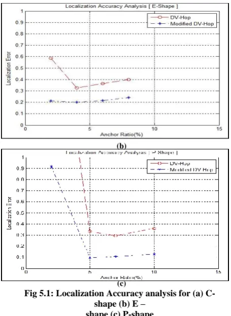
A. Anchor ratio Vs Localization error:

The below fig 5.1 shows the graph of anchor ratio Vs localization error. As anchor ratio is defined in section 4.3 it is the number of anchors per total number of nodes. So the anchor ratio must be less and for the network localization error also should be minimum. Based on both of these parameters the localization accuracy is decided. If localization error is less then it means that accuracy is more.

(a)

4.2

(b)

(c)

Fig 5.1: Localization Accuracy analysis for (a) C-shape (b) E –

shape (c) P-shape

B. Execution Time analysis:

The graphs for the execution time analysis are as shown in fig 5.2. In this analysis the time is measured in milliseconds (msec). This can also be called as algorithm run time or convergence time. For an efficient network the convergence time that is the time taken for the execution of algorithm should be less. For the proposed algorithm it is proved that the time is less.

(a)

(b)

Fig 5.2: Execution Time analysis for (a) C-shape (b) E – shape (c) P-shape

C. Median Hop Vs number of packets per node:

In fig 5.3 the diagrams of average hop versus number of packets per node. In a network the number of packets consumed should be less. If the packets per node are less then it will take less time for the communication. In the below graph for the modified DV-Hop the number of packets per node increases as the average hop increases.

(a)

Fig 5.3: Average Hop Vs Number of Packets analysis for (a) C-shape (b) E– shape (c) P-shape

D. Energy Consumption:

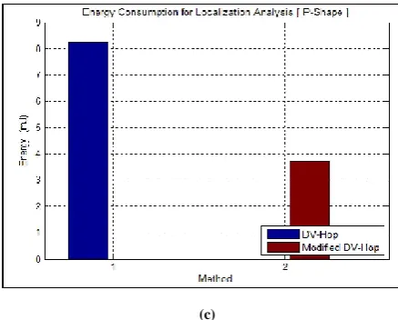
The diagram is as shown in the below fig 5.4 for all shapes. In any case of WSN the energy is an important parameter. The energy consumed by the network must be as less as possible. In the below graph for both DV-Hop and modified DV-Hop methods the energy consumed by the shapes are plotted. It is proved that modified DV-Hop consumes less energy.

(a)

(b)

(c)

Fig 5.4: Energy Consumption for Localization analysis for (a) C-shape (b) E – shape (c) P-shape

VI. CONCLUSION AND FUTURE WORK

In this proposed scheme modification over an improved Hop algorithm that is modified DV-Hop localization algorithm is proposed. For anisotropic networks like C, E and P shape the simulation is done. From the simulation results it is understood that more localization accuracy that is minimum localization error convergence time and energy consumption can be improved by the proposed algorithm. Simulation results are showed for C, E and P shapes. It is also explored the influence of the anchor nodes on the modified DV-Hop algorithm. From this it is understood that the number of anchor nodes could affect the convergence time and localization accuracy.

In the simulation results it is showed that localization accuracy is more, decreased convergence (execution) time and less energy consumption for the P-shape. So the modified DV-Hop Algorithm is better than previously proposed algorithm.

In the future work it can be simulated for three dimensional (3D) node deployment strategies. It can be further improved in localization accuracy by using other methods.

REFERENCES

[1] Dunfan Ye, Daoli Gong, Wei Wang, “Applications of Wireless Sensor Netroks in Environmental Monitoring”, IEEE, 2009.

[2] Soumya Simpi, Suresh Kuri, Praveen Kalkundri, “ Efficient Localizaztion Techniques for WSN –A survey”, International Journal of Advanced Reasearch in Compter and Communication engineering, Vol 6, 2017.

[3] Abhishek Kumar, Deepak Prashar,“Localization Techniques in Wireless Sensor Networks:A Review”,International journal of Advanced Research in Computer and Communication Engineering,vol 5, August 2016.

[4] Niharika Singh Matharu, “Localization Techniques in Wireless Sensor Networks:A Survey”, Journal of Network Communications and Emerging Technologies, vol 3 , August 2015.

3rd _{International conference on Recent trends in Computing}

2015(ICRTC-2015).

[6] Hongyang Chen, Kaoru Sezaki, Ping Deng,Hing Cheung So, “An Improved DV-Hop Localization Algorithm for Wireless Sensor Networks”, IEEE, 2008.

[7] Farrukh Shahzad, Tarek R. Sheltami, Elhadi M. Shakshuki, “Multi- Objective Optimization for a Reliable Localization Scheme in Wirelesssensor networks”, Journal of communications and Networks, vol 18, October 2016.

[8] Er Ram Dyal, Er varinderjit kaur, “Analyasis of Some localization algorithm in Wireless Sensor Networks”,International Journal of computer and organization Trends, Vol 11, Aug 2014.

[9] P.K Singh, Bharat Tripathi, Narendra Pal Singh,”Node Localization in Wireless Sensor Networks”, (IJCSIT) International Journal of Computer Science and Information Technologies, Vol. 2 (6) , 2011.

[10] Chuan Cai, Liang Yuan, “DV-Hop Localization Algorithm improvement of Wireless Sensor Network”, Journal of theoretical and Applied Information Technology, Vol 48, 28th Feburary 2013.

[11] Yu Hu, Xuemei, “An Improvement of DV-Hop Localization algorithm for wireless sensor networks”, springer, 28 June 2013.

[12] LI Nian-qiang, LI Ping,”A Range-Free Localization Scheme in Wireless Sensor Networks”, IEEE, 2008. [13] Shrawan Kumar, D.K.Lobiyal, “Improvement over

DV-Hop Localization Algorithm for Wireless Sensor Networks”, International Journal of Electrical, Computer, Energetic, [13]. Electronic and Communication Engineering, Vol4, 2013.

[14] Guangjie Han, Huihui Xu , Trung Q. Duong, Jinfang Jiang, Takahiro Hara,”Localization algorithms ofWireless Sensor Networks: a survey”, Springer Science+Business Media, LLC 2011.

[15] Azzedine boukerche, Horacio a. B. F. Oliveira, eduardo f. Nakamura, antonio a. F. Loureiro,”Localization Systems for Wireless Sensor Networks”, IEEE Wireless Communications, December 2007.

[16] U.Nazir, M. A. Arshad, N. Shahid, S. H. Raza,”Classification Of Localization algorithms for Wireless Sensor Network: A Survey”, 2012 International Conference on Open Source Systems and Technologies (ICOSST).

[17] S.B.Kotwal, Shekhar Verma, R.K. Abrol, “Approaches of Self Localization in Wireless Sensor Networks and Directions in 3D”, 2012.

[18] Diego Fco. Larios, Julio Barbancho, Fco. Javier Molina and Carlos Le´on “Localization method for low-power wireless sensor networks” Senior Member, IEEE, 2013.

[19] Cesare Alippi and Giovanni Vanini, “A RSSI-based and calibrated centralized localization technique for Wireless Sensor Networks”, in Proceedings of Fourth IEEE International Conference on Pervasive Computing and Communications Workshops (PERCOMW’06), Pisa, Italy, March 2006, pp. 301-305.

[20] Long Cheng, Chengdong Wu, Yunzhou Zhang, Hao Wu, Mengxin Li, Carten Maple,”A Survey of Localization in

Wireless Sensor Network”, Hindawi Publishing Corportation, pp.1-9,2012.

[21] Asma Mesumoudi, Mohammed Feham, Nabila Labraoui,” Wireless Sensor Netwaork Localization Algorithm: A Comprehensive Survey”, International Journal of Computer Networks and Communication (IJCNC) Vol.5, NO.6, November 2013.

[22] Nabil Ali Alrajeh, Maryam Bashir, Bilal shams,” Localization Techniques in Wireless Sensor Networks”, Hindawi Publising Corportation,pp.1-9,2013.

[23] Stefan Tomic, Ivan Mezei, "Improvements of DV-Hop localization algorithm for wireless sensor networks", Springer, 2015.

[24] Ashok Kumar, Narottam Chand, Vinod Kumar and Vinay Kumar, "Range Free Localization Schemes for Wireless Sensor Networks" , International Journal of Computer Networks & Communications (IJCNC) Vol.3, No.6, November 2011.

[25] Huang, Q, Selvakennedy, S. “A Range Free Localization Algorithm for Wireless Sensor Networks”. IEEE Vehicular Technology Conferences (VTC06), pp.349--353, Melbourne, Australia, 2006.

[26] Y.T.Chan, K.C.Ho,” A simple and Efficient Estimator for Hyperbolic Location”, IEEE, Vol 42, August 1994. [27] Jose.M. Alcala and Alvaro Hernadez, Victor Cionca,