Consolidation Of Soft Computing Approaches For Predictingthe Wheat Yield In India

Consolidation Of Soft Computing Approaches For

Predictingthe Wheat Yield In India

Surjeet Kumar, Manas Kumar Sanyal

Abstract— this paper prognosticates the production of wheat crop by developing a hybrid model through the combination of soft computing approaches. This material illustrates a brief study on the time series forecasting to predict the future data on the basis of the previous year data. The proposed model has been developed with the combination of Statistical Equations, Artificial Neural Network (ANN) and Genetic Algorithm (GA) to speculate the wheat production and to get more explicit outcomes. This model has been tested on the wheat production data of India from 1980 to 2018. Thereafter, by using statistical error computing techniques like Mean Square Error (MSE), Root Mean Square Error (RMSE) and Average Error, the Prediction Performances have been evaluated. It has been observed that due to the use of our proposed model compared to the Standalone Soft Computing, error prediction decreased.

Keyword —Statistical Equations, Artificial Neural Network (ANN), Genetic Algorithm (GA), Root Mean Square Error (RMSE), Mean Square Error (MSE) and Average Error.

————————————————————

1 I

After rice, wheat is an important cereal in India. This grain is mainly cultivated in the middle and western part of India. But the productivity of the wheat crop is not enough to feed India's huge population. Latest technology has an increasing effect on the growth of wheat production but still no fruitful results are seen.Like other agricultural products, wheat yield is also sensitive to multiple factors, which often relate to each other, directly and indirectly influence the crop production. Environmental factors, technological factors, plant variety, fertilizer‘s level are often considered.

By using different types of plant yield models, production performance can be optimized and stimulated. Accordingly, plant yield models may emerge the prognostic tools which can be a significant component of the precision farming and a vital component of Decision Support System (DSS).Recently, the use of Soft Computing analysis in the agricultural sector has increased.This often provides better analytical results compared to the classical statistical methods. Here, we have proposed ahierarchical non-linear regressive framework to determine the relationship between the crop yielding and sowing [7].

According to the above description, it appears necessary to attempt a research in order to get an optimum wheat yield assessment and prediction model through the soft computing assessment techniques which have not been developed yet. Thence, the following pilot study has been attempted to develop such model and to analyze it.The main goal of this paper is to structure a hybrid model byamplifyingthe precisenessof the projectionand extrapolationof the wheatcrop data. This new method is used on secondary time series data of wheatyield in India [3].

The reliabilityand consistencyof this estimationdepends on time series data.In agronomy, latesttechnologies are applied in

time series data to analysis and predict the upcomingresults on the basis of past data [1, 2].In Soft Computing, the Artificial Neural Network (ANN) is a frequently used method for forecasting in different fields of finance, education, production and agriculture [4]. The learning algorithm, like back-propagation algorithm, adjusts the network‘s weights and biases by calculating gradient of the error and then forecasts the error backward by the network to modify the weights and biases [5].Here, Artificial Neural Network is used to determine and to forecastthebuildingcost index for concreting structures on the basis of past records [6]. By using Population, Gross Domestic Product (GDP)and Vehicle-Km,the Genetic Algorithm

Transport Energy Demand Estimation model has

beenstructured [8]. Genetic algorithm finds the best equation to describethe temporal changes of monsoon in India at all times [9].Another technique for short-term load prediction with a lead time of one day is ANN and GA [10].Theunconstrained building optimization problems that are coupled of energy simulation program are also solvedby using Genetic Algorithm,[11].

The rest of this paperisorganized as: In section 2, Research and Methodologyare discussed. In section 3, Proposed Algorithm is canvassed by flow chart. In section 4, Results of the developed model isexplained. In section 5, Conclusion and the scope of the study is narrated and lastly the reference iselucidated in section 6.

2

R

M

Soft Computing Methods arefrequently applied to resolve manycritical problemsof thereal-life. In this study, we have used different types of Soft Computing Methodsto forecast and to build a hybrid model to get more accurate outcomes.

2.1 Statistical Equations

Statistical Equation is a crucial part of Soft Computing Analysis. We have employed different types of Statistical Equations like Polynomial, Linear, Gaussian, Fourier, Exponential and Sum of Sine and one of this equation is selected for prediction depends on the minimum error. ————————————————

 Surjeet Kumaris currently pursuing ph. D degree program in University of Kalyani, West Bengal, India. E-mail: [email protected]

Graph 1, it is clearly noticedthat Sum of Sine is the best fitted for wheat crop data set based on the Root Mean Square Error. The constant value, obtains from the Sum of Sine, isused to predict the future data on the basis of the actual data.

Sum of Sine, f(x) = a1*sin (b1*x+c1) (1) Where,a1, b1 and c1are constant values.

2.2 Artificial Neural Network

Artificial Neural Network (ANN) is a mathematical model. It simulates the formation and the applicative details of biological neural networks. The construction of Neural Network is similar to the human brain and this network consists of many processing components called neurons. After getting information from the surrounding neurons, neurons execute some calculations and pass the outcomes to the other neurons. Connections of neurons have associated some weights with them. The connection between two neurons can transmit signal from one to another Artificial Neuron. TheArtificial Neuron processes the received signal and then signal additional artificial neurons connected to it. Informationwhichis flowing across the network has an effect on the construction of ANN as neural network changes - or learns, in a sense - based on that input and output [13].

Three main layers of neural network are: Input, hidden and output layer. As represented graph2, two constant values (obtained From Sum of Sine) are adopted in input layer then three neurons are taken up in hidden layers and finally two optimum constant values are gotafter training in output layer. Throughout the training, Weights and bias are balanced in automated manneruntil it providesoptimal results. Constant(Sum of Sine) value provides more accurate predictive data set. Everyiterationshowsthe error ofpredictive data. Neural Network also provides the predictive data set. But still the validity of predictive data is based on the time series data.

2.3 Genetic Algorithm

Genetic algorithm (GA) is a group of evaluation based calculative models. This algorithm encodes a possible solution to a specified problem on an easily understandable data structure like chromosome, and uses recombination operators to this structure as to keep the finical information. GA is usually seen as function optimizer, even though the span of problems to which genetic algorithm has been used is wide-ranging.

The performance of a GA starts with a chromosomes‘ population (usually random). Then this structure is evaluated and reproductive opportunities are allocated in this way that the better solution given chromosomes of the target problem get more opportunities to ‗reproduce‘ than the poorer solution given chromosomes. On the basis of current population, ‗goodness‘ of the solution is usually defined [14].Generally, Genetic Algorithm uses binary (0, 1) notations. Thus, data have to be encoded into binary notation and this is stated as binary chromosome.

close parenthesis. However, longer lists will be formatted so that:

1. Selection operatorsareapplied to pick up solutions from the present population that isused in formation of the next population of the solutions. Roulette wheel method, which is formulated by Holland,is an elementary strategy of random selection [12].

2. Crossover process is used to mixthe ―genetic information‖ adopted from paired individuals through thecontrol of recombination operator. In the other way, Crossover randomly selectsthe pair of the best solution (Parent Chromosome) and interchanging them to produce a new child.Trial and Error method is used to detect the best result.

3. Mutation is done by using a bit-wise probabilistic method wherethe stated gene value if reversed from 0 to 1, and vice versa. Here, the effects of the mutation probability on search performancesarestudied through applications (trials) [11].

4. The fitness function is not only a function that is closely related to the designer‘s intentions but it also counts quickly.A fitness function has a specific type of objective function that is summarized as a single figure of merit, determines how close a given design solution is to achieve the set objectives. Therefore, individuals of Graph 1. Fitness of statistical equations

returned.In this study, Mean Absolute Percentage Error (MAPE) is applied as fitness function.

General equation of MAPE is as follow:

MAPE = 1/n ∑ [(│Actual Value – Forecasted Value│) / Actual Value] * 100. (2)

Where, n is number of fitted point of data set.

3

E

C

T

We are employingstatistical parameters to examine the accuracy of performances of different Soft Computing Approaches.

Mean Square Error (MSE) = ∑ni=1(Actual Value – Forecast Value) 2_/n

Mean Absolute Percentage error = ∑ni=1[mod (Ei-Fi)/Ei] *100/n

Where Ei=Actual value and Fi = forecast value.

Residual Analysis –

Absolute Residual = mod [Actual value – Forecast value] Mean Absolute Residual = mod [Actual value – Forecast value]/Actual value

4

P

A

H

M

B

S

C

T

5 R

D

5.1 First, we have shown the data prediction using different types of statistical equations in Table 1.

Table 1.

Year Produc- tion

Polyno- mial

Linear Fitting

Expone-ntial

Fourier Gaussian Sum of Sine 1980 31830 36273 56722.8 41127.23 1692.188 37365.4 35918.54

1981 36313 37866 55597.61 42107.27 3379.319 38712.36 37561.71

1982 37452 39459 55243.53 43110.67 5061.394 40085.02 39203.03

1983 42794 41052 55115.76 44137.97 6738.412 41482.7 40842.43

1984 45476 42645 54577.46 45189.76 8410.373 42904.67 42479.82

1985 44069 44238 53485.3 46266.61 10077.28 44350.09 44115.12

1986 47052 45831 52321.19 47369.12 11739.12 45818.08 45748.25

1987 44323 47424 51749.25 48497.9 13395.92 47307.7 47379.13

1988 46169 49017 52005.2 49653.58 15047.65 48817.92 49007.68

1989 54110 50610 52679.66 50836.8 16694.33 50347.65 50633.82

1990 49850 52203 53094.5 52048.21 18335.95 51895.73 52257.47

1991 55134 53796 52926.35 53288.49 19972.51 53460.94 53878.55

1992 55690 55389 52503.87 54558.33 21604.02 55041.97 55496.99

1993 57210 56982 52505.61 55858.43 23230.47 56637.47 57112.69

1994 59840 58575 53336.12 57189.51 24851.86 58246.02 58725.59

1995 65470 60168 54754.05 58552.3 26468.2 59866.13 60335.6

1996 62097 61761 56094.01 59947.58 28079.48 61496.24 61942.64

1997 69350 63354 56878.35 61376.1 29685.7 63134.75 63546.64

1998 66350 64947 57256.29 62838.66 31286.87 64779.98 65147.51

1999 71288 66540 57866.75 64336.07 32882.98 66430.22 66745.18

2000 76369 68133 59250.91 65869.17 34474.03 68083.69 68339.56

2001 69681 69726 61354.67 67438.8 36060.03 69738.55 69930.59

2002 72766 71319 63578.36 69045.83 37640.97 71392.95 71518.18

2003 65761 72912 65328.12 70691.15 39216.85 73044.94 73102.25

2004 72156 74505 66561.85 72375.69 40787.68 74692.59 74682.73

2005 68637 76098 67827.92 74100.36 42353.45 76333.88 76259.54

2006 69355 77691 69761.04 75866.14 43914.16 77966.8 77832.6

2007 75807 79284 72498.66 77673.99 45469.82 79589.27 79401.83

2008 78570 80877 75554.64 79524.92 47020.41 81199.22 80967.15

2009 80679 82470 78266.17 81419.96 48565.96 82794.54 82528.5

2010 80804 84063 80403.18 83360.16 50106.44 84373.1 84085.78

2011 86874 85656 82379.87 85346.59 51641.87 85932.77 85638.94

2012 94882 87249 84873.86 87380.35 53172.24 87471.41 87187.88

2013 93506 88842 88203.23 89462.58 54697.56 88986.87 88732.53

2014 95850 90435 92034.05 91594.43 56217.82 90477.01 90272.83

2015 86530 92028 95687.42 93777.08 57733.02 91939.69 91808.68

2016 87000 93621 98763.62 96011.74 59243.17 93372.79 93340.02

2017 98510 95214 101509.6 98299.65 60748.25 94774.2 94866.77

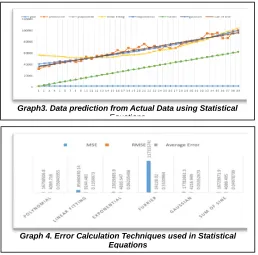
5.2 Determining the accuracy of the predicted data and Error Calculation Technique Using Statistical Equations Statistical

Equations have been used to predict the data set and to find the error by using error calculation techniques. Table 2 shows that Sum of Sine equation gives minimum error. So,Sum of Sine is the most suitable for wheat yield data predictionafter that we have to implementit in Artificial Neural Network.

5.3 Determining the Accuracy of the Predicted Data Using Statistical Equations

Here, Sum of Sineis indicated bymaroon red and the actual data is indicated by using orange color. Thedata prediction accuracy becomesmore accurate using Sumof Sine than the other statistical equations in Graph 3.Graph4, shows that accuracy of error calculation by using different statistical techniques.

5.4On the basis of minimum error, we have takenthe Sum of Sine prediction data. Then, the constant value is optimized using Artificial Neural Networkand more accurate prediction data set than the sum of sine data is

technique of the soft computing approach, brings more accuracy in prediction performance of the proposed hybrid model. All predicated data are shown in Table 3 and Error calculations are shown in Table 4.

Table 2. Methodsof Error calculation

Statistical

Equation MSE RMSE Average Error

Polynomial 16758506.8 4093.716 0.05043355

Linear Fitting 85460430.14 9244.481 0.1359973 Exponential 22029385.9 4693.547 0.06235406 Furrier 1171557414 34228.02 0.5530964 Gaussian 17782661.3 4216.949 0.05352673 Sum of Sine 16723971.9 4089.495 0.04978739

Graph3. Data prediction from Actual Data using Statistical Equations

Graph 4. Error Calculation Techniques used in Statistical Equations

Table 3. Data prediction using Soft Computing Techniques

year production sum of sine ANN prediction GA Prediction 1980 31830 35918.5404 35939.22732 31829.948

1981 36313 37561.71042 37590.60737 36313.677

1982 37452 39203.03362 39240.12066 37451.438

1983 42794 40842.42928 40887.68529 42793.146

1984 45476 42479.8168 42533.21944 45476.292

1985 44069 44115.11568 44176.64139 44069.063

1986 47052 45748.24551 45817.86953 47051.29

1987 44323 47379.12599 47456.82235 44322.646

1988 46169 49007.67694 49093.41846 46169.185

1989 54110 50633.81828 50727.5766 54110.633

1990 49850 52257.47007 52359.2156 49850.122

1991 55134 53878.55245 53988.25445 55134.415

1992 55690 55496.98575 55614.61224 55691.721

1993 57210 57112.69036 57238.2082 57209.545

1994 59840 58725.58687 58858.96172 59839.596

1995 65470 60335.59596 60476.7923 65471.034

1996 62097 61942.63847 62091.6196 62096.939

1997 69350 63546.63539 63703.36344 69350.522

1998 66350 65147.50785 65311.94376 66350.253

1999 71288 66745.17714 66917.28069 71287.154

2000 76369 68339.56471 68519.29451 76368.504

2001 69681 69930.59217 70117.90566 69681.741

2002 72766 71518.18128 71713.03476 72766.74

2003 65761 73102.25399 73304.60259 65759.536

2004 72156 74682.73241 74892.53011 72157.818

2005 68637 76259.53884 76476.73846 68637.847

2006 69355 77832.59574 78057.14898 69356.367

2007 75807 79401.82577 79633.68319 75808.159

2008 78570 80967.15178 81206.26278 78571.591

2009 80679 82528.4968 82774.80967 80679.951

2010 80804 84085.78406 84339.24596 80803.609

2011 86874 85638.937 85899.49397 86873.661

2012 94882 87187.87925 87455.47621 94882.58

2013 93506 88732.53465 89007.1154 93506.303

2014 95850 90272.82725 90554.33451 95850.79

2015 86530 91808.68132 92097.05668 86529.597

2016 87000 93340.02135 93635.20532 87000.438

2017 98510 94866.77205 95168.70403 98509.899

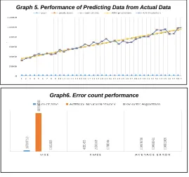
5.5In the Hybrid model, the predicated data of Genetic algorithm and the actual data are overlapped. Actual data ispresented bysaffron color and the predicated data of Genetic algorithm is indicatedby azure blue inGraph 5. The reliabilityof the prediction performance becomes more accurate using Neural Network with Genetic Algorithm. Error counting accuracy is shown in Graph 6.

6

C

This paper represents an effort tospeculate wheat crop production using the Soft Computing Techniques.The error is further rectified by the ANN on the basis of properly optimized constant value of Sum of Sine. Thus, we get predicted average error is 0.0496848. Finally, Genetic algorithm is applied to obtain more reliable data prediction and the average error of this performance is 0.00001005. It is observed that the efficiency of the proposed hybrid model becomes better in performance. In the future, we will experiment with different soft computing methods to maybe get more accurate results in crop production and weather data.

7

R

[1] Time series data analysis of ENR construction cost index, A. Baabak, ASCE 136(11) (2010), 1227-1237.

[2] W. Enders, Applied econometric time series, Wiley, New York, 2008.

[3] Wheat data source

https://www.indexmundi.com/agriculture/?country=in&co mmodity=corn&graph=production.

[4] M. Adya, F. Collopy, ―How Effective are Neural Networks at Forecasting and Prediction‖, Journal of Forecasting, vol. 17, no. 5–6, 1998, pp. 481–495.

[5] ―Acceleration of Back Propagation through Initial Weight Pre-training with Delta Rule‖, in: Proceedings of the IEEE International Conference on Neural Networks, vol. 1, pp. 580– 585, San Fransisco, CA, 1993.

[6] ―Estimation and prediction of construction cost index using neural network, time series and regression‖, Yasser Elfahham, Alexandria engineering journal (2019).

[7] Statistical processing of experimental data, Meeloun, Militky 1996, univerzita Pardubice, Czech Republic ISBN 80-7194-075-5.

[8] ―Genetic algorithm approach to estimate transport energy demand in Turkey‖, Article in energy policy 33(1):89-98 • January 2005.

[9] ―Forecasting summer rainfall over India using genetic algorithm‖, C. M. Kishtawal, Sujit Basu, Falguni Patadia, P. K. Thapliyal, geophysical researchletters, vol. 30, no. 23,2203. [10] ―Short Term Electric Load Forecasting using Neural Network

and Genetic Algorithm‖, International Journal of Applied Information Systems 2016,Foundation of Computer Science (fcs), ny, USA.

[11] ―Selecting the most efficient genetic algorithm sets in solving unconstrained building optimization problem‖, Ali Alajmi and Jonathan Wright, International Journal of Sustainable Built Environment,(2014) 3, 18-26.

[12] ―Genetic algorithms in search, optimization, and machine learning‖, Addison-Wesley Publishing Company, Reading, Goldberg DE (1989).

[13] ―Neural Networks for Prediction of Oil Production‖, Leyla Muradkhanli, conference paper IFAC Papers online 51-30 (2018) 415–417.

[14] ―Statistics and Computing - A Genetic Algorithm tutorial‖, Springer June 1994, Volume 4, Issue 2, PP 65-85.

Table 4. Error CalculationUsing Different Soft ComputingTechniques

Purposed Method MSE RMSE Average Error

sum of sine 16723971.9 4089.495 0.04978739 Artificial Neural

Network (ANN) 653502260 25563.69 0.04968481 Genetic

Algorithms (GA) 0.621805 0.788546 0.00001005

Graph 5. Performance of Predicting Data from Actual Data