for Left Censored Burr Type III Distribution
Navid Feroze
Department of Statistics, Government Post Graduate College Muzaffarabad, Azad Kashmir, Pakistan
Muhammad Aslam
Department of Statistics, Rifa International University, Islamabad, Pakistan [email protected]
Tabassum Naz Sindhu
Department of Statistics, Quad-i-Azam University, Islamabad, Pakistan [email protected]
Abstract
Burr type III is an important distribution used to model the failure time data. The paper addresses the problem of estimation of parameters of the Burr type III distribution based on maximum likelihood estimation (MLE) when the samples are left censored. As the closed form expression for the MLEs of the parameters cannot be derived, the approximate solutions have been obtained through iterative procedures. An extensive simulation study has been carried out to investigate the performance of the estimators with respect to sample size, censoring rate and true parametric values. A real life example has also been presented. The study revealed that the proposed estimators are consistent and capable of providing efficient results under small to moderate samples.
Keywords: Maximum likelihood estimation, loss functions, prior distribution, Bayes risks.
1. Introduction
Burr type iii distribution has also not received the sizeable attention of the analysts yet. It can be used as an alternative to many lifetime distributions including Weibul and Burr type xii distributions. Recently, Abd-Elfattah and Alharbey (2012) have discussed the Bayesian and maximum likelihood estimation of the parameters of Burr type iii distribution under doubly censored samples, but the process they have used to calculate MLE is not very efficient which has also been suggested by the simulation results. Further, they have not derived the expressions for the Fisher information matrix. We have proposed a logical methodology to calculate the MLEs and to derive elements of Fisher information matrix on the basis of left censored samples.
The probability density function (pdf) of the Burr type iii distribution is:
1
11
f x x x ; x0, , 0. (1) where and are the shape parameters of the distribution. It can be observed that the pdf of this distribution is very close to the Burr type xii distribution. With little transformations the Burr type xii distribution can be obtained. However, the Burr type iii distribution can cover wider region for the skewness and kurtosis plane. The cumulative distribution function for the Burr type iii distribution can be written as:
1
F x x (2)
The left censored data is very likely to occur in survivor analysis. It can happen where an event of interest has already occurred at the observation time, but it is not known exactly when. For example, the situations including: the infection with a sexually-transmitted disease such as HIV/AIDS, onset of a pre-symptomatic illness such as cancer and time at which teenagers begin to drink alcohol can lead to left censored data. In case of left censored samples, we can only observe those individuals whose event time is greater than some truncation point. This truncation point may or may not be the same for all individuals. For example, in case of actuarial life studies, the individuals those died in the womb are often ignored. Another example: suppose you wish to study how long patients who have been hospitalized for a heart attack survive taking some treatment at home. In such situations, the starting time is often considered to be the time of the heart attack. Only those patients who survive their stay in hospital are able to be included in the study. The more illustrations on left censoring can be seen from: Lawless and Jerald (2003), Sinha (2006), Asselineau et al. (2007), Antweller and Taylor (2008), Thompson et al. (2011), Feroze and Aslam (2012b) and Sindhu et al. (2013). These studies motivated the authors to conduct the current analysis under left censored samples.
2. Materials and Methods
This section contains the derivation of maximum likelihood estimates, elements of Fisher information matrix, variance covariance matrix and confidence intervals for the parameters of the Burr type iii distribution under left censored samples. The limiting behavior of the Fisher information matrix has also been discussed.
2.1. Maximum likelihood estimation
discussed in the following. Let X r1...X n be the last n r ordered statistics from the Burr type iii distribution. Then, the likelihood function for the sample of n r left censored sample can be defined as:
( 1)
( )
1 , , , , , n r r i i rL F x f x
Using (1) and (2), it can be written as:
11
( 1) ( ) ( )
1
, 1 1
n
r n r
r i i
i r
L x x x
(3)The log-likelihood function is given as:
( 1)
( )
( )
1 1
, ln 1 ln 1 ln 1 ln 1
n n
r i i
i r i r
l r x n r x x
(4)
The normal equations to derive the MLEs of parameters and are:
( 1)
( )
1
ln 1 ln 1 0
n
r i
i r
l n r
r x x
(5)
( 1) (
1) ( )
( ) ( )
1 1
( 1) ( )
ln ln
ln 1 0
1 1
n n
r r i i
i
i r i r
r i
r x x x x
l n r
x x x
(6)From (5), the MLE of can be derived as a function of that can be denoted as:
( 1)
( )
1 ˆ
ln 1 ln 1
n
r i
i r
n r
r x x
(7)It is observed from (6) that the MLE of the parameter cannot be obtained in closed form. It can be obtained by solving a one dimensional optimization problem. A simple fixed point iteration algorithm can be used to solve this optimization problem. Firstly, the parameter in log-likelihood (4) has been replaced by its MLE given in (7) the resultant log-likelihood becomes:
( 1)( 1) ( ) ( 1) ( )
1 1
( ) 1
( 1) ( )
1
ln 1
ln ln
ln 1 ln 1 ln 1 ln 1
1 ln 1 ln
ln 1 ln 1
r
n n
r i r i
i r i r
n
i n
i r i r
r i
i r
n r r x n r
l n r n r
r x x r x x
n r x
r x x
1
( )
1
n
i
x
After some simplifications it can be presented as:
( )
( )
( 1)
( )
1 1 1
ln ln 1 1 ln ln ln 1 ln 1
n n n
i i r i
i r i r i r
l n r x x n r r x x
(8)MLE of can be obtained by maximizing (8)with respect to and it is unique. Most of the standard iterative process can be used for finding the MLE. We propose the following simple algorithm. If ˆ is the MLE of , then it is obvious from l'
0thatˆ
satisfies the following fixed point type equation; g
Where
1 ( 1) ( 1) ( ) ( )
1
( 1) ( )
( ) ( ) ( )
1 1 ( )
( 1) ( )
1 ln ln 1 1 ln 1 ln 1
ln 1 ln 1
n
r r i i
n n i r
r i
i i
i n
i r i r i
r i
i r
rx x x x
x x
x x
g x
n r x
r x x
(9)The iterated result of the above function has been considered as an MLE of and denoted by ˆ . Now the approximate MLE of has been incorporated in (7) to obtain the MLE of.
2.2. Approximate Fisher information matrix
In this section, the efforts have been made to derive the elements of the Fisher information matrix for the parameters of the Burr type iii distribution under left censored samples. The variance covariance matrix for the parameters of the Burr type iii distribution can be obtained by inverting the Fisher information matrix. The Fisher information matrix can be defined as:
2 2 2 2 2 2 , l l I l l (10)The equations for the elements of the Fisher information matrix can be written as:
2
2 2
l n r
(11)
2
( 1) ( 1) ( ) ( ) 1
( 1) ( )
ln ln
1 1
n
r r i i
i r
r i
rx x x x
l x x
(12)
2
1 2
2 2 2
( 1) ( 1) ( 1) ( 1) ( 1) ( 1) 2
1 2
2 2 2
( ) ( ) ( ) ( ) ( ) ( ) 2
1
ln 1 ln 1
1 ln 1 ln 1
r r r r r r
n
i i i i i i
i r
l
r x x x x x x
n r
x x x x x x
Now, the expected values of the (12) and (13) require the distribution of the th
i order statistics from the Burr type iii distribution which can be written as:
1 1
1
( ) , 1 ( ) 1 1 ( ) ( ) 1 ( )
n i i
i n i i i i i
g x C x x x x
0x( )i
1
1( ) , ( ) ( )
0
1 1
n i i j
j
i n i i i
j
n i
g x C x x
j
(14)where
,
!
1 ! !
n i
n C
i n i
The expectations necessary to derive the elements of the Fisher information matrix are given as:
1
( ) ( ) ( ) , 0
1 1
ln 1 1 2 ,
n i j
i i i n i
j
n i
x x x C B i j
j
(15)
2 1
( ) ( ) ( ) ,
0
1 1 1 1
ln 1 1 2 , 2
n i j
i i i n i
j
n i
x x x C B i j i j
j
(16)
2 2 2
( ) ( ) ( ) ,
0
1 1 1 1
ln 1 1 3 , 3
n i j
i i i n i
j
n i
x x x C B i j i j
j
(17)where, B x y
, is a standard beta function and
' z z z is a digamma function.
Now using (15), (16) and (17), the components of the Fisher information matrix become:
2
2 2
l n r
2 1
, 1 ,
0 1 0
1 1 1 1 1
1 2 , 1 1 2 ,
n r n n i
j j
n r n i
j i r j
n r n i
l
rC B r j C B i j
j j
2 1 2 , 1 2 2 0 1 2 , 1 01 1 1 1 1
1 2 , 1 2 1
1 1 1 1 1
1 3 , 1 3 1
n r j n r j n r j n r j n r l n r
r C B r j r j
j n r
r C B r j r j
j
, 1 0 , 1 01 1 1 1
1 1 2 , 2
1 1 1 1
1 1 3 , 3
n n i j
n i i r j
n n i j
n i i r j
n i
C B i j i j j
n i
C B i j i j j
The variance covariance matrix can be obtained by inverting the Fisher information matrix as:
1 ˆ ˆ ˆ, , ˆ ˆ ˆ, V Cov I Cov V covariance matrix can be used to construct the approximate confidence intervals for the said parameters. The approximate confidence intervals for and as discussed by Wu and Kus (2009) are:
/2
ˆ Zk V ˆ
and ˆZk/ 2 V
ˆ where kis the level of significance.2.3. Limiting Fisher information matrix
This section discusses the asymptotic efficiencies and limiting information matrix when
r
n converges to, say, p which lies in (0,1). According to Gupta et al. (2004), for the
left censored observations at the time pointT, the limiting Fisher information matrix can be written as
11 12 21 22
( , ) b b
I
b b
(18)
where
( ln ( , ))( ln ( , )) ( ; )
ij
i j
T
b r y r y f y dy
and ( , ), ( , ) ( ; )( ; )
f y r y
F y
the
reversed hazard function. Zheng and Gastwirth (2000) have shown that for location and scale family, the Fisher information matrix for Type-I and Type-II (both for left and right censored data) are asymptotically equivalent. They further described that for general case (not for location and scale family) the results for Type-II censored data (both for left and right) of the asymptotic Fisher information matrices are very difficult to obtain. We cannot obtain the explicit expression for the limiting Fisher information matrix for Burr type iii distribution under left censored samples as it does not belong to the location and scale family. Numerically, we have studied the limiting behavior of the Fisher information matrix by taking n5000 (assuming it is very large) and compare them with the different small samples and different ‘p’ values. The numerical results have been presented in section (3).
3. Numerical Results
This section covers the discussions regarding the results of the simulation study along with real life example. The samples of size n = 20, 50, 100, 150 and 200 have been generated by inverse transformation technique using the function X
U1/ 1
1/where U Uniform 0,1
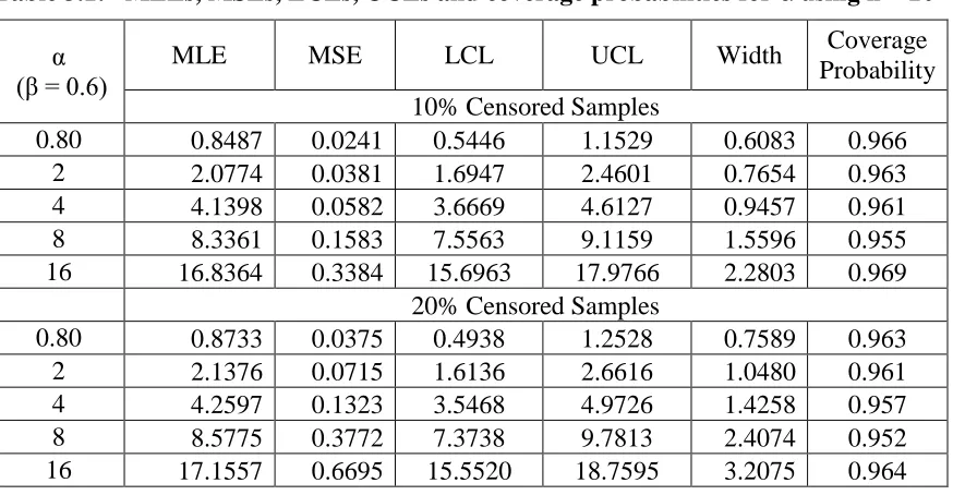
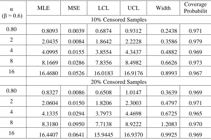
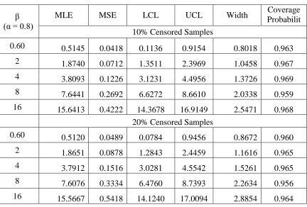
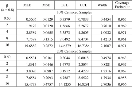
. The parametric space contains:square errors (MSEs); while, the performance of the confidence intervals have been discussed on the basis of the widths of the intervals along with corresponding coverage probabilities. For the whole parametric space of the we have assumed 0.6 and for the entire parametric space of we assumed0.8. The entries in the tables below are the average of the results under 10000 replications. The maximum likelihood estimates (MLEs), MSE, 95% lower confidence limits (LCL), upper confidence limits (UCL), width of the confidence limits and associated coverage probabilities (proportion of the intervals containing the true parametric values to the total (10000) intervals) have been presented in the tables.
Table 3.1: MLEs, MSEs, LCLs, UCLs and coverage probabilities for α using n = 20
α (β = 0.6)
MLE MSE LCL UCL Width Coverage
Probability 10% Censored Samples
0.80 0.8487 0.0241 0.5446 1.1529 0.6083 0.966
2 2.0774 0.0381 1.6947 2.4601 0.7654 0.963
4 4.1398 0.0582 3.6669 4.6127 0.9457 0.961
8 8.3361 0.1583 7.5563 9.1159 1.5596 0.955
16 16.8364 0.3384 15.6963 17.9766 2.2803 0.969
20% Censored Samples
0.80 0.8733 0.0375 0.4938 1.2528 0.7589 0.963
2 2.1376 0.0715 1.6136 2.6616 1.0480 0.961
4 4.2597 0.1323 3.5468 4.9726 1.4258 0.957
8 8.5775 0.3772 7.3738 9.7813 2.4074 0.952
16 17.1557 0.6695 15.5520 18.7595 3.2075 0.964
Table 3.2: MLEs, MSEs, LCLs, UCLs and coverage probabilities for α using n = 50
α (β = 0.6)
MLE MSE LCL UCL Width ProbabilitCoverage
y 10% Censored Samples
0.80 0.8303 0.0149 0.5912 1.0694 0.4782 0.968
2 2.0694 0.0274 1.7452 2.3936 0.6484 0.964
4 4.1216 0.0405 3.7273 4.5159 0.7886 0.961
8 8.1956 0.0749 7.6592 8.7320 1.0728 0.957
16 16.6402 0.1821 15.8038 17.4766 1.6727 0.972
20% Censored Samples
0.80 0.8544 0.0253 0.5427 1.1661 0.6234 0.965
2 2.0866 0.0405 1.6922 2.4810 0.7888 0.962
4 4.1558 0.0633 3.6625 4.6490 0.9865 0.957
8 8.3472 0.1635 7.5546 9.1398 1.5852 0.954
Table 3.3: MLEs, MSEs, LCLs, UCLs and coverage probabilities for α using n = 100
α (β = 0.6)
MLE MSE LCL UCL Width ProbabilitCoverage
y 10% Censored Samples
0.80 0.8176 0.0095 0.6262 1.0090 0.3827 0.970
2 2.0369 0.0154 1.7936 2.2802 0.4865 0.972
4 4.0925 0.0253 3.7808 4.4043 0.6235 0.969
8 8.1912 0.0570 7.7235 8.6590 0.9355 0.971
16 16.5512 0.1168 15.8815 17.2209 1.3394 0.971
20% Censored Samples
0.80 0.8484 0.0158 0.6023 1.0945 0.4922 0.967
2 2.0766 0.0251 1.7659 2.3873 0.6214 0.970
4 4.1381 0.0396 3.7480 4.5282 0.7802 0.965
8 8.3327 0.1204 7.6527 9.0127 1.3600 0.968
16 16.6660 0.1737 15.8492 17.4829 1.6337 0.966
Table 3.4: MLEs, MSEs, LCLs, UCLs and coverage probabilities for α using n = 150
α (β = 0.6)
MLE MSE LCL UCL Width Coverage
Probabilit y 10% Censored Samples
0.80 0.8093 0.0039 0.6874 0.9312 0.2438 0.971
2 2.0435 0.0084 1.8642 2.2228 0.3586 0.979
4 4.0995 0.0155 3.8554 4.3437 0.4882 0.969
8 8.1669 0.0286 7.8356 8.4982 0.6626 0.973
16 16.4680 0.0526 16.0183 16.9176 0.8993 0.967
20% Censored Samples
0.80 0.8327 0.0086 0.6508 1.0147 0.3639 0.969
2 2.0604 0.0150 1.8206 2.3003 0.4797 0.971
4 4.1335 0.0294 3.7973 4.4698 0.6725 0.965
8 8.3180 0.0950 7.7138 8.9222 1.2083 0.970
Table 3.5: MLEs, MSEs, LCLs, UCLs and coverage probabilities for α using n = 200
α (β = 0.6)
MLE MSE LCL UCL Width ProbabilitCoverage
y 10% Censored Samples
0.80 0.8050 0.0023 0.7114 0.8985 0.1871 0.982
2 2.0325 0.0048 1.8971 2.1679 0.2708 0.976
4 4.0645 0.0068 3.9031 4.2260 0.3230 0.976
8 8.1232 0.0144 7.8879 8.3585 0.4706 0.981
16 16.4293 0.0330 16.0734 16.7851 0.7117 0.982
20% Censored Samples
0.80 0.8242 0.0040 0.7002 0.9481 0.2478 0.979
2 2.0173 0.0042 1.8908 2.1438 0.2529 0.974
4 4.0200 0.0057 3.8724 4.1676 0.2953 0.972
8 8.0949 0.0127 7.8736 8.3161 0.4425 0.978
16 16.1903 0.0234 15.8903 16.4904 0.6001 0.977
Table 3.6: MLEs, MSEs, LCLs, UCLs and coverage probabilities for β using n = 20
β (α = 0.8)
MLE MSE LCL UCL Width Coverage
Probabilit y 10% Censored Samples
0.60 0.5145 0.0418 0.1136 0.9154 0.8018 0.963
2 1.8740 0.0712 1.3511 2.3969 1.0458 0.967
4 3.8093 0.1226 3.1231 4.4956 1.3726 0.969
8 7.6441 0.2692 6.6272 8.6610 2.0338 0.959
16 15.6413 0.4222 14.3678 16.9149 2.5471 0.968
20% Censored Samples
0.60 0.5120 0.0489 0.0784 0.9456 0.8672 0.960
2 1.8651 0.0878 1.2843 2.4459 1.1616 0.965
4 3.7912 0.1516 3.0281 4.5542 1.5261 0.965
8 7.6076 0.3334 6.4760 8.7393 2.2634 0.956
Table 3.7: MLEs, MSEs, LCLs, UCLs and coverage probabilities for β using n = 50
β (α = 0.8)
MLE MSE LCL UCL Width ProbabilitCoverage
y 10% Censored Samples
0.60 0.5409 0.0223 0.2480 0.8338 0.5858 0.966
2 1.9140 0.0392 1.5258 2.3022 0.7763 0.968
4 3.8526 0.0774 3.3074 4.3978 1.0904 0.969
8 7.7470 0.1563 6.9721 8.5219 1.5498 0.961
16 15.6624 0.3364 14.5256 16.7992 2.2737 0.972
20% Censored Samples
0.60 0.5383 0.0279 0.2110 0.8656 0.6546 0.963
2 1.9049 0.0521 1.4575 2.3522 0.8947 0.966
4 3.8342 0.1007 3.2122 4.4562 1.2440 0.965
8 7.7100 0.2066 6.8192 8.6009 1.7817 0.958
16 15.5877 0.4421 14.2844 16.8910 2.6066 0.967
Table 3.8: MLEs, MSEs, LCLs, UCLs and coverage probabilities for β using n = 100
β (α = 0.8)
MLE MSE LCL UCL Width Coverage
Probabilit y 10% Censored Samples
0.60 0.5606 0.0129 0.3379 0.7833 0.4454 0.965
2 1.9172 0.0320 1.5666 2.2677 0.7010 0.969
4 3.8589 0.0655 3.3573 4.3605 1.0032 0.971
8 7.7598 0.1315 7.0492 8.4704 1.4213 0.961
16 15.6882 0.2872 14.6379 16.7386 2.1007 0.971
20% Censored Samples
0.60 0.5531 0.0161 0.3044 0.8018 0.4974 0.963
2 1.8914 0.0446 1.4773 2.3054 0.8281 0.967
4 3.8070 0.0987 3.1912 4.4229 1.2316 0.967
8 7.6554 0.2093 6.7587 8.5522 1.7934 0.958
Table 3.9: MLEs, MSEs, LCLs, UCLs and coverage probabilities for β using n = 150
β (α = 0.8)
MLE MSE LCL UCL Width ProbabilitCoverage
y 10% Censored Samples
0.60 0.5838 0.0064 0.4265 0.7412 0.3147 0.968
2 1.9581 0.0162 1.7084 2.2078 0.4993 0.970
4 3.9027 0.0399 3.5113 4.2941 0.7828 0.971
8 7.8478 0.0749 7.3113 8.3844 1.0731 0.963
16 15.8662 0.1572 15.0892 16.6433 1.5540 0.974
20% Censored Samples
0.60 0.5760 0.0110 0.3706 0.7814 0.4108 0.965
2 1.9317 0.0299 1.5928 2.2707 0.6780 0.968
4 3.8502 0.0738 3.3177 4.3828 1.0652 0.967
8 7.7423 0.1496 6.9841 8.5005 1.5164 0.960
16 15.6529 0.3267 14.5326 16.7732 2.2406 0.969
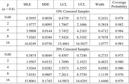
Table 3.10: MLEs, MSEs, LCLs, UCLs and coverage probabilities for β using n = 200
β (α = 0.8)
MLE MSE LCL UCL Width Coverage
Probability 10% Censored Samples
0.60 0.5955 0.0038 0.4739 0.7171 0.2431 0.978
2 1.9777 0.0095 1.7867 2.1686 0.3818 0.982
4 3.9808 0.0144 3.7452 4.2163 0.4712 0.984
8 7.9263 0.0384 7.5424 8.3102 0.7678 0.973
16 16.0249 0.0756 15.4861 16.5637 1.0777 0.983
20% Censored Samples
0.60 0.5874 0.0049 0.4507 0.7240 0.2733 0.975
2 1.9507 0.0152 1.7090 2.1923 0.4833 0.980
4 3.9264 0.0282 3.5973 4.2555 0.6582 0.980
8 7.8181 0.0807 7.2611 8.3750 1.1139 0.970
Table 3.11: Elements of variance-covariance matrix including V
ˆ and
ˆ, ˆCov for 10% censored data, the covariance terms have been
presented in parenthesis
β Sample Size
(α = 0.8) 20 50 100 150 200 5000
0.6 0.0181 0.0126 0.0088 0.0037 0.0022 0.0018
(0.0834) (0.0663) (0.0554) (0.0334) (0.0202) (0.0161)
2 0.0281 0.0195 0.0136 0.0057 0.0034 0.0027
(0.1106) (0.0879) (0.0735) (0.0443) (0.0269) (0.0214)
4 0.0398 0.0276 0.0192 0.0080 0.0049 0.0039
(0.1162) (0.0923) (0.0772) (0.0465) (0.0282) (0.0225)
8 0.0662 0.0459 0.0319 0.0133 0.0081 0.0064
(0.2138) (0.1698) (0.1421) (0.0855) (0.0519) (0.0413)
16 0.0743 0.0515 0.0359 0.0150 0.0091 0.0072
(0.6689) (0.5314) (0.4445) (0.2677) (0.1624) (0.1292)
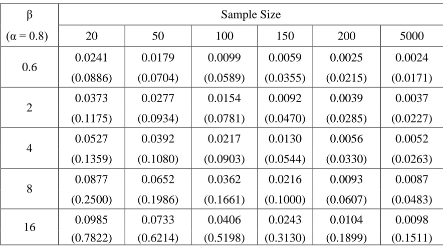
Table 3.12: Elements of variance-covariance matrix including V
ˆ and
ˆ, ˆCov for 20% censored data, the covariance terms have been
presented in parenthesis
β Sample Size
(α = 0.8) 20 50 100 150 200 5000
0.6 0.0241 0.0179 0.0099 0.0059 0.0025 0.0024
(0.0886) (0.0704) (0.0589) (0.0355) (0.0215) (0.0171)
2 0.0373 0.0277 0.0154 0.0092 0.0039 0.0037
(0.1175) (0.0934) (0.0781) (0.0470) (0.0285) (0.0227)
4 0.0527 0.0392 0.0217 0.0130 0.0056 0.0052
(0.1359) (0.1080) (0.0903) (0.0544) (0.0330) (0.0263)
8 0.0877 0.0652 0.0362 0.0216 0.0093 0.0087
(0.2500) (0.1986) (0.1661) (0.1000) (0.0607) (0.0483)
16 0.0985 0.0733 0.0406 0.0243 0.0104 0.0098
Table 3.13: Elements of variance-covariance matrix including V
ˆ and
ˆ, ˆCov for 10% censored data, the covariance terms have been
presented in parenthesis
α Sample Size
(β = 0.6) 20 50 100 150 200 5000
0.8 0.0233 0.0143 0.0103 0.0074 0.0050 0.0040
(0.0834) (0.0663) (0.0554) (0.0334) (0.0202) (0.0161)
2 0.0361 0.0221 0.0160 0.0115 0.0078 0.0062
(0.1451) (0.0733) (0.0531) (0.0382) (0.0259) (0.0207)
4 0.0510 0.0313 0.0226 0.0163 0.0110 0.0088
(0.1678) (0.0848) (0.0614) (0.0442) (0.0300) (0.0240)
8 0.0849 0.0520 0.0377 0.0271 0.0184 0.0147
(0.3085) (0.1560) (0.1130) (0.0813) (0.0551) (0.0441)
16 0.0953 0.0584 0.0423 0.0304 0.0206 0.0165
(0.9654) (0.4881) (0.3536) (0.2545) (0.1725) (0.1380)
Table 3.14: Elements of variance-covariance matrix including V
ˆ and
ˆ, ˆCov for 20% censored data, the covariance terms have been
presented in parenthesis
α Sample Size
(β = 0.6) 20 50 100 150 200 5000
0.8 0.0367 0.0291 0.0244 0.0147 0.0089 0.0071
(0.1162) (0.0588) (0.0426) (0.0306) (0.0208) (0.0166)
2 0.0478 0.0314 0.0181 0.0187 0.0089 0.0085
(0.1541) (0.0779) (0.0565) (0.0406) (0.0275) (0.0220)
4 0.0676 0.0445 0.0256 0.0265 0.0126 0.0120
(0.1782) (0.0901) (0.0653) (0.0470) (0.0319) (0.0255)
8 0.1125 0.0739 0.0426 0.0440 0.0210 0.0199
(0.3278) (0.1657) (0.1201) (0.0864) (0.0586) (0.0469)
16 0.1263 0.0830 0.0479 0.0495 0.0236 0.0223
(1.0257) (0.5186) (0.3757) (0.2704) (0.1833) (0.1466)
on the performance of the interval estimation, that is, the bigger sample sizes lead to the smaller widths of the confidence intervals and larger coverage probabilities. This simply indicates that the estimators of the parameters are consistent. The coverage probabilities do not provide any pattern with respect to change in the true parametric values. However, it is good to see that coverage probabilities regarding all the confidence intervals are greater than 0.95 (which are greater than concerned confidence coefficient) that indicates the reliability of the interval estimation. The confidence intervals for parameter ( ) are skewed to right, while the intervals regarding parameter () are left aligned. As a natural consequence, the increased censoring rate results in: slower convergence of estimates, inflated MSEs, wider confidence intervals and smaller coverage probabilities. However, it has been observed that the affects of the left censored observations are not that much severe in case of bigger sample sizes. Further for fixed sample size and censoring rate, the higher actual values of the parameters impose a negative impact on the performance (in terms of MSEs, convergence rate and widths of confidence intervals) of the estimates. It leads to the conclusion that the estimation of extremely large values of the parameters of the Burr type iii distribution may become difficult and the Fisher information matrix may be the decreasing function of the parameters. But the moderate to huge sample sizes can face off this problem.
In the tables 3.11-3.14, we have discussed the limiting behavior of the variance covariance matrix obtained by inverting the fisher information matrix given in (11). As the analytical results of the Fisher information matrix for n cannot be obtained, we have calculated the entries of the Fisher information/variance covariance matrix by taking n = 5000 (extremely large). Different levels of the censoring rate have been employed for the analysis. The covariance terms have been presented in the parenthesis. It is interesting to note that efficiency of the estimates in the moderately large samples is close to that in limiting case. The variance covariance terms are decreasing by increasing the sample size. This simply suggests that the parameters of the Burr type iii distribution can efficiently be estimated by using moderately large left censored samples.
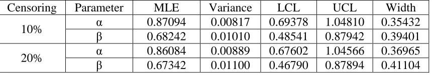
Now we consider the analysis of real life data set regarding the breaking strengths of 64 single carbon fibers of length 10, presented Lawless and Jerald (2003). The idea has been to see whether the results and properties of the estimators, explored by simulation study, are applicable to a real life situation. We have used the Kolmogorov-Smirnov and chi square tests to see whether the data follow the Burr type III distribution. These tests say that the data follow the Burr type III distribution at 5% level of significance with p-values 0.2173 and 0.7352 respectively. The results of the analysis have been reported in the following table.
Table 3.15: Estimation under real life data
Censoring Rate
Parameter MLE Variance LCL UCL Width
10% α 0.87094 0.00817 0.69378 1.04810 0.35432
β 0.68242 0.01010 0.48541 0.87942 0.39401
20% α 0.86084 0.00889 0.67602 1.04566 0.36965
The estimated values of the parameter () are relatively higher than those of parameter (). The real life analysis replicated the patterns observed under simulation study in a sense that the variances associated with MLEs of are smaller than those for MLEs of
. The widths of confidence intervals are also smaller in case of estimation for parameter . Similar patterns were observed for the near values of and in case of simulation study.
4. Conclusion
The article aims to discuss the maximum likelihood estimation of the parameters for Burr type iii distribution under left censored samples. The behavior and performance of the estimates have been investigated with respect to sample sizes, true parametric values and censoring rates. The findings of the study suggest that even the small samples sizes with higher censoring rates are closely related to the limiting figures of the variance covariance matrix. It leads to the conclusion that the approximate variance covariance matrix can effectively be used for analysis of the unknown parameters of the Burr type iii distribution. It further indicates that the proposed maximum likelihood point and interval estimates can efficiently be applied to the real life situations using moderate sample sizes. The results of the real life data analysis further strengthened these arguments. The study is useful for scientists from different fields dealing with analysis of left censored failure time data.
References
1. Abd-Elfattah, A. M., Alharbey, A. H. (2012). Bayesian Estimation for Burr Distribution Type III Based on Trimmed Samples, ISRN Applied Mathematics, 3, 1-18.
2. Antweller, R. C., Taylor, H. E. (2008). Evaluation of Statistical Treatments of Left-Censored Environmental Data using Coincident Uncensored Data Sets: I. Summary Statistics, Environ. Sci. Technol., 42, 3732 3738.
3. Asselineau, J., Thiebaut, R., Perez, P. et al. (2007). Analysis of Left-Censored Quantitative Outcome: Example of Procalcitonin Level, Rev Epidemiol Sante Publique, 55(3), 213-20.
4. Burr, W. I. (1942). Cumulative Frequency Distribution, Annals of Mathematical Statistics, 13, 215-232.
5. Dasgupta, R. (2011). On The Distribution of Burr with Applications, Sankhya B, 73, 1-19
6. Feroze, N., Aslam, M. (2012b). On Bayesian Analysis of Burr Type VII Distribution under Different Censoring Schemes, International Journal of Quality, Statistics, and Reliability, 3, 1-5
7. Feroze, N., Aslam, M. (2012a). Bayesian Analysis of Burr Type X Distribution under Complete and Censored Samples, International Journal of Pure and Applied Sciences and Technology, 11(2), 16-28
9. Gupta, R. D., Gupta, R. C., Sankaran, P. G. (2004). Fisher Information In Terms Of the (Reversed) Hazard Rate Function, Communication in Statistics: Theory and Methods, 33, 3095-3102.
10. Lawless, J. F, Jeral, F. (2003). Statistical Models and Methods for Lifetime Data. Second Edition, University of Waterloo.
11. Nadar, M., Alexandros, P. (2011). Bayesian Analysis for the Burr Type XII Distribution Based on Record Values, Statistica, 71(4), 421-435.
12. Shao, Q. (2004a). Notes on Maximum Likelihood Estimation for the Three-Parameter Burr XII Distribution, Computational Statistics and Data Analysis, 45, 675-687.
13. Shao, Q., Wong, H., Xia, J. (2004b). Models for Extremes Using the Extended Three Parameter Burr XII System with Application to Flood Frequency Analysis,
Hydrological Sciences Journal des Sciences Hydrologiques, 49, 685-702.
14. Silva, G. O., Ortega, E. M. M., Garibay, V. C. et al. (2008). Log-Burr XII Regression Models with Censored Data, Computational Statistics and Data Analysis, 52, 3820-3842.
15. Sindhu. T. N., Aslam, M. and Feroze, N. (2013). Bayes Estimation of the Parameters of the Inverse Rayleigh Distribution for Left Censored Data. ProbStat Forum, 6, 42-59.
16. Sinha, P., Lambert, M. B., Trumbull, V. L. (2006). Evaluation of Statistical Methods for Left-Censored Environmental Data with Nonuniform Detection Limits, Environ Toxicol Chem., 25(9), 2533-40.
17. Soliman, A. A. (2002). Reliability Estimation in a Generalized Life Model with Application to the Burr-XII, IEEE Tran. on Reliability, 51, 337-343.
18. Soliman, A. A. (2005). Estimation of Parameters of Life from Progressively Censored Data Using Burr-XII Model, IEEE Transactions on Reliability, 54, 34-42.
19. Thompson, E. M., Hewlett, J. B., Baise, L. G. (2011). The Gumbel Hypothesis Test for Left Censored Observations Using Regional Earthquake Records as an Example, Nat. Hazards Earth Syst. Sci., 11, 115-126.
20. Wahed, A. S. (2006). Bayesian Inference Using Burr Model under Asymmetric Loss Function: An Application to Carcinoma Survival Data, Journal of Statistical Research, 40(1), 45-57.
21. Wu, J. W., Yu, H. Y. (2005). Statistical Inference about the Shape Parameter of the Burr Type XII Distribution Under The Failure-Censored Sampling Plan,
Applied Mathematics and Computation, 163(1), 443-482.
22. Wu, S. J., Chen, Y. J., Chang, C. T. (2007). Statistical Inference Based On Progressively Censored Samples with Random Removals from the Burr Type XII Distribution, Journal of Statistical Computation and Simulation, 77, 19-27.
23. Wu, S., Kus, C. (2009). On Estimation Based on Progressive First-Failure-Censored Sampling, Computational Statistics and Data Analysis, 53, 3659-3670. 24. Zheng, G., Gastwirth, J. L. (2000). Where Is The Fisher Information in an