DOI: http://dx.doi.org/10.15282/ijsecs.3.2017.9.0031
PARAMETER-LESS SIMULATED KALMAN FILTER
Nor Hidayati Abdul Aziz1,2, Zuwairie Ibrahim2, Nor Azlina Ab. Aziz1
and Saifudin Razali2
1Faculty of Engineering and Technology, Multimedia University
Bukit Beruang, Melaka, Malaysia
2Faculty of Electrical and Electronics Engineering, Universiti Malaysia Pahang
Pekan, Pahang, Malaysia
e-mail: [email protected], [email protected] [email protected], [email protected]
ABSTRACT
Simulated Kalman Filter (SKF) algorithm is a new population-based metaheuristic optimization algorithm. In the original SKF algorithm, three parameter values are assigned during initialization, the initial error covariance, P(0), the process noise, Q, and the measurement noise, R. Further studies on the effect of P(0), Q and R values suggest that the SKF algorithm can be realized as a parameter-less algorithm. Instead of using constant values suggested for the parameters, this study uses random values for all three parameters, P(0), Q and R. Experimental results show that the parameter-less SKF managed to converge to near-optimal solution and performs as good as the original SKF algorithm.
Keywords: Optimization, Simulated Kalman Filter, parameter-less
INTRODUCTION
Simulated Kalman Filter (SKF) was first introduced in by Ibrahim et al. (2015) as an optimizer for unimodal optimization problems. The benchmarking of the SKF algorithm later has been extended to simple multimodal, hybrid and composite functions of the CEC 2014 benchmark suite (Ibrahim et al., 2016). Since then, the algorithm has been subjected to various adaptations and applications. These include extensions of the SKF algorithm by Md. Yusof et al. (2015) to deal with combinatorial optimization problems. The original SKF algorithm has been applied to find the optimal path of a 14-hole drill path optimization problem (Abdul Aziz, Ab. Aziz, Ibrahim and Razali, 2016) while the discrete type of SKF algorithm has been subjected to solve Airport Gate Allocation Problems (AGAP) by Mohd Azmi et al. (2016) and feature selection problem for EEG peak detection by Adam et al. (2016). Hybrid versions of the SKF algorithm have been introduced by Muhammad et al. (2015) by hybridizing the SKF algorithm with PSO algorithm, and later with the GSA algorithm (Muhammad et al., 2016). All these studies suggest SKF is a good global optimizer.
130
towards the overall performance. Genetic Algorithm (GA) is another example of algorithms that has many setting parameters. Parameters in GA include the probability of mutation and crossover, and the selection procedure (Holland, 1975). Particle Swarm Optimization (PSO) on the other hand, despite being easy to understand, also has 3 parameters to be tuned (Kennedy & Eberhart, 1995). Some classical algorithms, such as Tabu Search (TS) (Glover, 1986) and Simulated Annealing (SA) (Kirkpatrick, 2012), has at least 1 or 2 parameters required tuning. Usage of such algorithms requires some preliminary tuning computation of the parameters before applying them to solve an optimization problem.
Another option is to offer some default values for the parameters. Covariance Matrix Adaptation Evolution Strategy (CMA-ES) by Hansen, Ostermeier and Gawalczyk (1995) is an example of an algorithm which offers some default parameter values to the users. These values are claimed to be applicable to any optimization problems in hand. Self-tuning parameters, like what has been introduced in Differential Evolution (DE) (Storn & Price, 1997), is another alternative solution. Ultimately parameter-free algorithms such as Black Hole (Hatamlou, 2013) and Symbiotic Organisms Search (SOS) (Cheng & Prayogo, 2014) are desirable. Therefore, this research is conducted as an attempt to introduce a parameter-less version of Simulated Kalman Filter (SKF) algorithm.
THE ORIGINAL AND PARAMETER-LESS SKF ALGORITHM
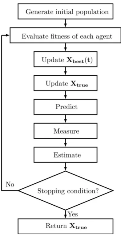
The Simulated Kalman Filter (SKF) algorithm is a population-based algorithm inspired by the estimation capability of the Kalman Filter. The SKF algorithm is illustrated in Figure 1. Consider a population of N agents, the SKF algorithm starts with the initialization of the agents’ estimated state, X(0) = {X1(0), X2(0), … , XN-1(0), XN(0)}.
The initial estimated state of an agent, i, is defined as Xi(0) = {Xi1(0), Xi2(0), … , Xid -1(0), X
id(0)} where d refers to the problem’s dimension. The initial estimated state of the
agents, X(0), are randomly distributed within the search space of the problem. Besides
X(0), the initial error covariance, P(0), the process noise, Q, and the measurement noise,
R, are also initialized during this stage.
After initialization, the initial solution of each agent is evaluated using the fitness function of the problem. According to the type of the optimization problem, the agent with the best fitness in an iteration, t, is recorded as Xbest(t). The best-so-far
solution on the other hand, is called Xtrue. For minimization problem, Xtrue is updated
only if the fitness of Xbest (t) is less than the fitness of Xtrue. While for maximization
problem, Xtrue is updated only if the fitness of Xbest (t) is more than the fitness of Xtrue.
Next, is the prediction step. During this step, the predicted state of each agent, ( 1)
d i t
X , and its corresponding predicted error covariance are updated using the following time-update equations:
| 1
d d
i t t i t
X X (1)
| 1
After that, is the measurement step. In SKF, measurement for each agent is simulated in such a way that the measured values lie in an area surrounding the predicted value, as given by Eq. (3) with randid U
0,1 .( ) ( | 1) sin( 2 ) ( | 1)
d d d d
i t i t t randi i t t true
Z X X X (3)
This simulated measurement process helps to promote exploration, while at the same time, create balance between the exploration and exploitation in SKF.
Finally is the estimation step. During this step, Kalman gain, K(t), is first computed as follows:
( ) ( | 1) / ( | 1)
K t P t t P t t R (4)
Kalman gain act as a weighted average between the prediction and measurement during estimation. Then, the estimated state of the agent for the next time step, d( 1)
i t
X , and
the corresponding error covariance are calculated using the measurement-update equations as follows:
( 1) ( | 1) ( ) ( ) ( | 1)
d d d d
i t i t t K t i t i t t
X X Z X (5)
( 1) 1 ( ) ( | 1)
P t K t P t t (6)
132
Figure 1. SKF algorithm
The original SKF algorithm suggested the parameter P(0), Q and R to be given the value of 1000, 0.5 and 0.5 respectively. However, this study proposes that these parameter settings can be excluded. In this study, normally distributed random number, defined in the range of between 0 to 1, with a mean of 0.5 is suggested whenever a parameter value is needed, generated for every agent in every dimension, denoted as
d i randn .
In the proposed parameter-less SKF, during initialization, the initial error covariance, P(0), is set to be randnid. Then, during prediction, Eq. (7) is used instead of
Eq. (2).
( | 1) ( )
d d d
i i i
P t t P t randn (7)
And finally, during estimation, Eq. (8) is used to replace Eq. (4), and subsequently Eq. (9) is used replacing Eq. (6).
( ) ( | 1) / ( | 1)
d d d d
i i i i
( 1) 1 ( ) ( | 1)
d d d
i i i
P t K t P t t (9)
EXPERIMENTAL EVALUATION AND DISCUSSION
In order to evaluate the performance of the proposed parameter-less SKF algorithm, the algorithm is subjected to 30 benchmark functions from CEC 2014’s benchmark suite by Liang, Qu and Suganthan (2013). Note that all CEC 2014 benchmark functions are minimization problems and have the same search space of [-100,100] for all dimensions. The search agents in SKF were initialized randomly within the search space for all benchmark functions in a uniform distribution. 100 agents are used in the experiment. For each run of the experiment, the stopping condition is set at 10,000 number of function evaluations, and the experiment is being repeated for 50 times.
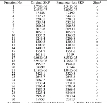
To evaluate the performance of the proposed parameter-less SKF algorithm, the average performance from 50 independent runs of each experiment were calculated and compared with the performance of the original SKF under the same experimental settings. Table 1 shows the comparison of the average value calculated over 50 runs between the original SKF and the parameter-less SKF algorithm. The sign is used to point which algorithm is better for each benchmark problem. However, this finding is far from conclusive.
134
Table 2. The Wilcoxon Signed-Rank Test
R+ R
-Original SKF vs Parameter-less SKF 199 264
For the Wilcoxon signed-rank test, the R+ and R- values were calculated and those values were compared to the threshold value obtained from the Wilcoxon statistical table considering 30 benchmark problems. Since both R+ and R- values are greater than the threshold value, which is 137, the finding suggests there is no significant difference between the results produced by both algorithms.
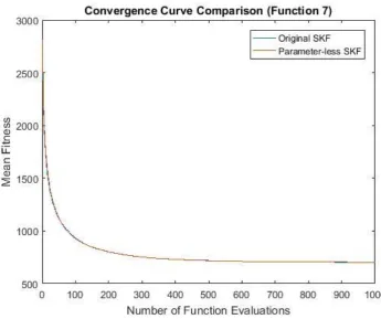
This finding is consistent when we compare the convergence curves produced by the original SKF algorithm and the convergence curves produced by the parameter-less SKF algorithm. Figure 2 below shows an example of the convergence curves produced by both algorithms in solving for function no. 7, a simple multimodal benchmark problem (Shifted and Rotated Griewank’s), which looks pretty much identical. Both algorithms managed to converge to a near optimal value in a similar pattern from start to finish.
Table 1. Performance comparison between the original SKF algorithm with parameter-less SKF algorithm
Function No. Original SKF Parameter-less SKF Sign*
1 4.70E+06 4.54E+06 >
2 2.45E+07 7.00E+07 <
3 18148 17492 >
4 532.77 544.25 <
5 520.01 520.01 =
6 633.44 632.76 >
7 700.25 700.35 <
8 807.98 809.13 <
9 1059.1 1058.7 >
10 1335.2 1360.2 <
11 6249.4 6209.8 >
12 1200.2 1200.2 =
13 1300.6 1300.6 =
14 1400.3 1400.3 =
15 1551.7 1551.6 >
16 1619.1 1619 >
17 9.08E+05 8.55E+05 >
18 6.94E+06 1.36E+07 <
19 1950.2 1944.8 >
20 34799 33544 >
21 1.19E+06 1.04E+06 >
22 3429.1 3320.8 >
23 2645.7 2645.8 <
24 2667.2 2664.2 >
25 2730.4 2731.8 <
26 2766.4 2782.4 <
27 3883.3 3869.4 >
28 7223.4 6846.6 >
29 5997.8 8030.4 <
30 19753 20513 <
Figure 2. Convergence curves comparison for function no. 7
CONCLUSION
A parameter-less SKF algorithm is successfully introduced. This proposed algorithm is tested for all types of optimization problems in the CEC2014 benchmark suite (unimodal, simple multimodal, hybrid and composition functions) and proven able to reach near-optimal solution without any significant degradation as compared to the original SKF algorithm. This enhancement enables users to use the SKF algorithm directly without the need to tune the parameters when solving for any specific optimization problem in the future.
ACKNOWLEDGEMENT
136
REFERENCES
Abdul Aziz, N. H., Ab. Aziz, N. A., Ibrahim, Z. & Razali, S. (2016). A Kalman Filter approach to PCB drill path optimization problem. IEEE Conference on Systems, Process and Control, 33–36.
Adam, A., Ibrahim, Z., Mokhtar, N., Shapiai, M. I., Mubin, M. & Saad, I. (2016). Feature selection using angle modulated simulated Kalman filter for peak classification of EEG signals. , SpringerPlus, 5(1580).
Cheng, M. Y. & Prayogo, D. (2014). Symbiotic organisms search: a new metaheuristic optimization algorithm. Journal of Computers & Structures, 139, 98–112.
Glover, F. (1986). Future paths for integer programming and links to artificial intelligence. Computers and Operations Research, 13, 533–549.
Hansen, N., Ostermeier, A. & Gawelczyk, A. (1995). On the adaptation of arbitrary normal mutation distributions in evolution strategies: the generating set adaptation. 6th International Conference on Genetic Algorithms, 57–64.
Hatamlou, A. (2013). Black hole: A new heuristic approach to data clustering.
Information Sciences, 222, 175-184. doi: 10.1016/j.ins.2012.08.023
Holland, J. H. (1975). Adaptation in natural and artificial systems. Ann Arbor: University of Michigan Press.
Ibrahim, Z., Abdul Aziz, N. H., Ab. Aziz, N. A., Razali, S., Shapiai, M. I., Nawawi, S. W. & Mohamad, M. S. (2015). A Kalman Filter approach for solving unimodal optimization problems. ICIC Express Letters, 9(12), 3415–3422.
Ibrahim, Z., Abdul Aziz, N. H., Ab. Aziz, N. A., Razali, S & Mohamad, M. S. (2016). Simulated Kalman Filter: A Novel Estimation-Based Metaheuristic Optimization Algorithm. Advance Science Letters, 22(10), 2941–2946.
Kalman, R. E. (1962). A new approach to linear filtering and prediction problems.
Trans. ASME-J. Basic Eng, 82(Series D), 35–45.
Kennedy, J. & Eberhart, R. (1995). Particle swarm optimization. IEEE Int. Conf. on Neural Network, 1972–1978.
Kirkpatrick, S., Gelatt, C. & Vecchi, M. (2012). Optimization by simulated annealing.
Science, 220, 671–680.
Liang, J. J., Qu, B. Y. & Suganthan, P. N. (2013). Problem definitions and evaluation criteria for the CEC 2014 special session and competition on single objective real-parameter numerical optimization. Tech. Rep. 201311.
Md Yusof, Z., Ibrahim, Z., Ibrahim, I., Mohd Azmi, K. Z., Ab. Aziz, N. A., Abdul Aziz, N. H., & Mohamad, M. S. (2015). Angle Modulated Simulated Kalman Filter algorithm for combinatorial optimization problems. ARPN Journal of Engineering and Applied Sciences, 11(7), 4854-4859.
Md Yusof, Z., Ibrahim, Z, Ibrahim, I, Mohd Azmi, K. Z., Ab. Aziz, N. A., Abdul Aziz, N. H., & Mohamad, M. S. (2015). Distance Evaluated Simulated Kalman Filter algorithm for combinatorial optimization problems. ARPN Journal of Engineering and Applied Sciences, 11(7), 4904-4910.
Md Yusof, Z., Ibrahim, I., Satiman, S. N., Ibrahim, Z., Abdul Aziz, N. H., & Ab. Aziz, N. A., (2015) BSKF: Binary Simulated Kalman Filter. 3rd International Conference on Artificial Intelligence, Modelling and Simulation, 77-81.
problem using angle modulated simulated Kalman filter. 3rd National Conf. Postgraduate Research, 875–885.
Muhammad, B., Ibrahim, Z., Ghazali, K. H., Mohd Azmi, K. Z., Ab. Aziz, N. A., Abdul Aziz, N. H., & Mohamad, M. S. (2015). A new hybrid Simulated Kalman Filter and Particle Swarm Optimization for continuous numerical optimization problems. ARPN Journal of Engineering and Applied Sciences, 10(22), 17171-17176.
Muhammad, B., Ibrahim, Z., Mohd Azmi, K. Z., Abas, K. H., Ab. Aziz, N. A., Abdul Aziz, N. H., & Mohamad, M. S. (2016). Four different methods to hybrid simulated Kalman filter (SKF) with gravitational search algorithm (GSA). 3rd National Conf. Postgraduate Research, 854–864.