Sample Holding Time Reevaluation

(1)

Sample Holding Time

Reevaluation

(2)

(3)

EPA/600/R-05/124 October 2005 www.epa.gov

Sample Holding Time

Reevaluation

Contract No. 68-D-99-011 Task Order No. 18 (ORD-01-005)

Prepared for

Brian A. Schumacher, Ph.D. U.S. Environmental Protection Agency National Exposure Research Laboratory

Environmental Sciences Division 944 East Harmon Avenue Las Vegas, Nevada 89119

Prepared by

Battelle Memorial Institute Pacific Northwest Division

Post Office Box 999 Battelle Boulevard Richland, Washington 99352

C.C. Ainsworth, V.I. Cullinan, E.A. Crecelius, K.B. Wagnon, and L.A. Niewolny

(4)

(5)

Notice

The information in this document has been funded wholly by the United States Environmental Protection Agency under contract number 68-D-99-011 to Battelle Memorial Institute. It has been subjected to the Agency’s peer and administrative review and has been approved for publication as an EPA document. Mention of trade names or commercial products does not constitute endorsement or recommendation by EPA for use.

(6)

(7)

Executive Summary

The project’s overall objective was to investigate the stability of selected contaminants in soil/sediment samples as a function of holding time prior to extraction. Contaminants of interest centered on SVOCs; particularly polyaromatic hydrocarbons (PAHs), polychlorinated biphenyls (PCBs), and pesticides, Cr(VI), and several heavy metals. Contaminant specific objectives were:

1. Determine if selected SVOC contaminant concentrations in soil/sediment changed with

time when held in storage beyond their established extraction maximum holding times (MHTs) under current preservation techniques and at -20°C;

2. Determine if Cr(VI) concentrations change when held in storage beyond their established

MHTs under current preservation techniques and at -20°C;

3. Determine if extracted Cr(VI) concentrations change when held beyond the analysis

MHT (24-h) when held in the dark at room temperature (~20°C) or 4°C;

4. Determine if air-drying soil samples will adversely impact hot acid extractable heavy

metal concentrations.

Test soils/sediments from contaminated sites were identified, collected and homogenized prior to extraction by SW-846 methods. After homogenization, soil/sediment samples were stored under designated conditions and extracted at multiples of the current MHT (depending on the

contaminant, multiples of MHT were between 0.5 and 12). Analyses of contaminant

concentrations were performed in accordance with SW-846 methodologies. Results of these extractions were evaluated by a progression of four distinct analyses to elucidate possible decreases in concentration of an analyte (lines of evidence). First, the magnitude and variability of the concentration was used to suggest a level of the signal to noise ratio; second, a t-test of the

H0:overall mean equal to or greater than the Day 0 mean was used to provide a level of relevance

to observed change; third, a regression against time was used to estimate a rate of change; and fourth, a nonparametric upper and lower bound based on the Day 0 quartiles was used to provide an alternative measure of relevance to the potential change through time. Ultimately; however, linear regression analysis was utilized to estimate the time required to observe a specific percent change in the extractable concentration.

The estimated number of days until a 5% decrease in Cr(VI) concentration from the estimated intercept would be observed was greater than 140 days for all sediments/soils tested. The results of this study suggest that the recoveries of matrix spike and control extracts are key to

determining stability of Cr(VI) in the solid materials to be extracted and the extracts themselves. In all cases, when the recovery of the matrix spike and control samples was good (within

acceptable parameters), the stability of Cr(VI) in the sediment/soil and extract solutions (stored under proper conditions) appear to be longer than the current MHT specified in SW-486. For the 17 PAH compounds that were quantified in three different soils/sediments, a holding

time of 100 days at either 4oC or -20oC would result in no more than a 20% decrease in

(8)

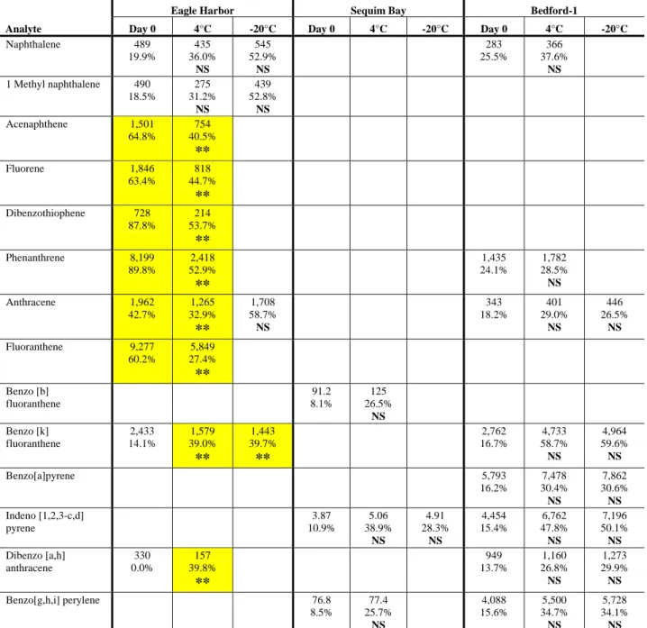
different compounds and in different soils/sediments. The major consideration in sediment holding time appears, from these studies, to be the number of aromatic rings (or molecular weight) of the PAH of interest. Only the Eagle Harbor soil appeared to have significant loss to

PAHs for samples stored at 4oC as compared to samples stored at -20oC. The loss of up to 50%

occurred for compounds with relatively low molecular weights, including acenaphthene, fluorene, dibenzothiophene, phenanthrene and anthracene. These results confirmed a previous study that demonstrated freezing sediment/soil reduced the loss of low molecular weight (low number of rings) PAHs.

For the three PCB Aroclor mixtures and the seven congeners that were quantified in three

different soils/sediments, a holding time of 260 days at 4oC and 281 days at -20oC would result

in not more than a 20% decrease in concentration. An indication of the stability of the PCBs in the three soil/sediments that were studied is the very small difference in the mean concentration for all data across time at two storage temperatures. In almost every case, the concentrations for

the -20oC samples are slightly greater, about 10% or less, than for the 4oC mean. This could be

interpreted that about 10% more PCBs are lost during the 5.6 month storage time at 4oC than at

-20oC. Given the 25% coefficient of variation (CV) metric for replicate precision; however, it is

unlikely that this 10% difference could be accurately quantified.

For the 10 pesticides that were quantified in four different soils/sediments, a holding time of 217

days at 4oC and 299 days at -20oC would result in not more than a 20% decrease in

concentration. These holding times are far greater than the current MHT specified in SW-846. In

almost every case, the mean concentrations for the -20oC samples are within a few percent of the

4oC mean. This could be interpreted as less than 5% of the pesticides studied are lost during the

5.6 month storage time of samples at 4oC compared to storage at -20oC.

Extractable metal concentrations were not effected significantly by a holding time of up to 364 days or by the air drying treatment. All data sets exhibited fairly tight CVs across the holding times. The CV data suggests that no chemically significant change in concentration occurred during the 364 day holding time and the pooled data exhibited no significant difference between moist or dry sample handling. These results suggest that it would take a minimum of 709 days before the acid-extractable As, Cu, Pb, or Zn concentration would be reduced by 20%.

(9)

List of Tables

Table Page

1-1 Soil/sediment sample preservation, and holding times, and extract preservation, and

holding times... 2

1-2 Changes made in Method 3060... 2

2-1 Available soils/sediments... 6

2-2 Comparison of analysis of variance and regression assuming six time points for chemical analysis, two replicate analyses at each time, and a linear relationship... 6

2-3 PAH analyte list ... 10

2-4 PCB (Aroclors and Congeners) and chlorinated pesticide analyte list ... 11

2-5 Summary of general data quality objectives ... 16

3-1 Chromate extraction study soil/sediment properties ... 18

3-2 Cr(VI) analyses of three Cr(VI) spiked Bedford-6 soil extracts ... 20

3-3 Chromate [Cr(VI)] (mg/kg) one-sample t-test of the null hypothesis Ho: the sample is from a population with the mean equal to or greater than the Day 0 mean ... 20

3-4 P-values for the significance of the lack-of-fit and the slope from the linear regression and the best fit simple linear model parameters on the natural log scale for Cr(VI) ... 23

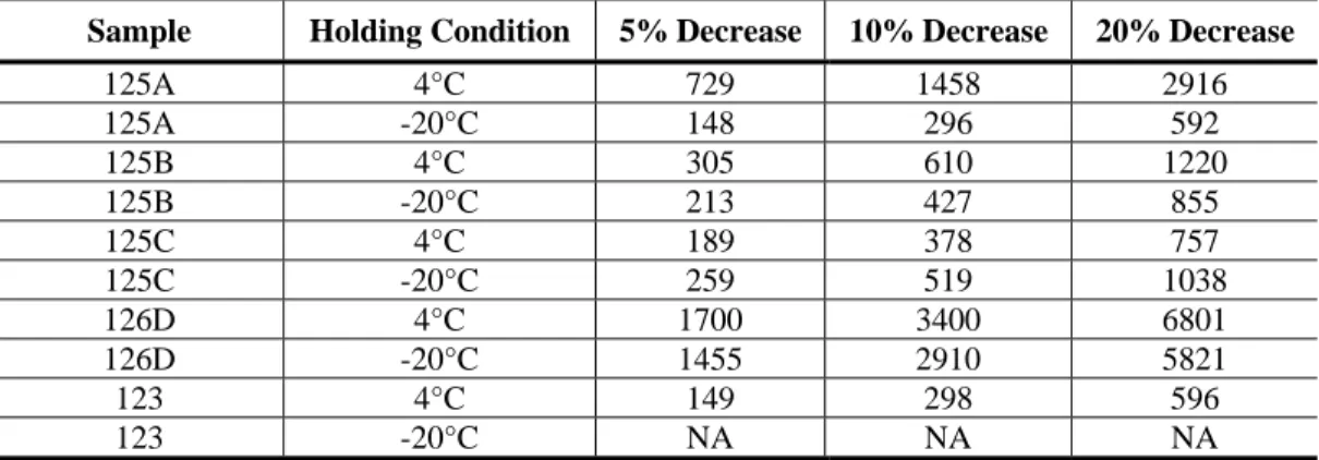
3-5 The estimated number of days until a given percentage decrease from the intercept for Cr(VI) (MHT=28 days) ... 24

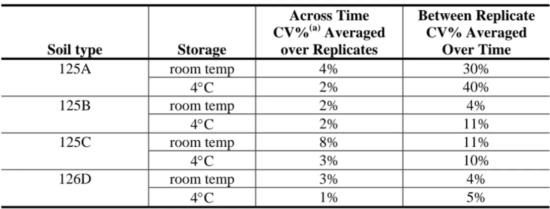
3-6 Average CV% over time and within replicates for the Cr(VI) extracts ... 28

3-7 Simple linear regression analysis corrected for baseline only ... 28

3-8 Estimated number of days to achieve a given percentage change in concentration using the regression model of the background corrected data... 30

3-9 SVOC extraction study soil/sediment properties ... 30

3-10 Mean concentration (ng/g) and coefficient of variation (CV) for all data across time accepted for analysis (including statistical outliers) ... 31

3-11 PAHs (ng/g) one-sample t-test of the null hypothesis Ho: the sample is from a population with the mean equal to or greater than the Day 0 mean from Appendix B for the Eagle Harbor soil ... 33

3-12 PAHs (ng/g) one-sample t-test of the null hypothesis Ho: the sample is from a population with the mean equal to or greater than the Day 0 mean from Appendix B for the SQ-1 sediment... 34

3-13 PAHs (ng/g) one-sample t-test of the null hypothesis Ho: the sample is from a population with the mean equal to or greater than the Day 0 mean from Appendix B for the Bedford-1 soil ... 36

(12)

Table Page 3-14 P-values for the significance of the lack-of-fit and the slope from the linear regression

and the best fit simple linear model parameters on the natural log scale for PAHs for

Eagle Harbor soil and each holding condition ... 37 3-15 P-values for the significance of the lack-of-fit and the slope from the linear regression

SQ-1 sediment and each holding condition ... 38 3-16 P-values for the significance of the lack-of-fit and the slope from the linear regression

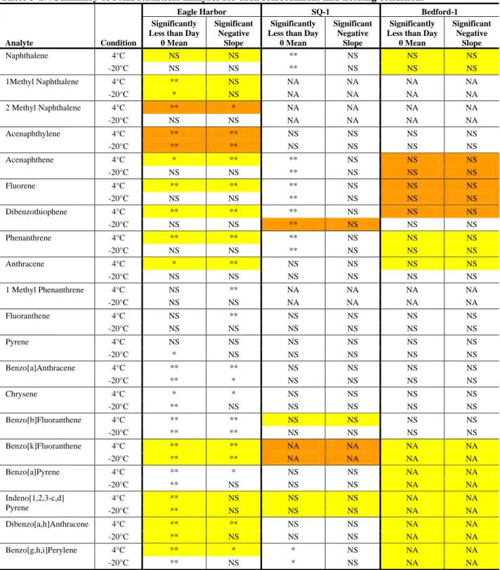
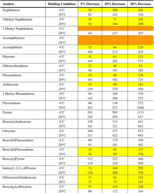
Bedford-1 soil and each holding condition ... 39 3-17 Summary of PAH statistical analyses for each soil/sediment and holding condition ... 40 3-18 The estimated number of days until a given percentage decrease from the intercept for

PAHs (MHT=14 days) from Eagle Harbor soil. ... 42 3-19 The estimated number of days until a given percentage decrease from the intercept for

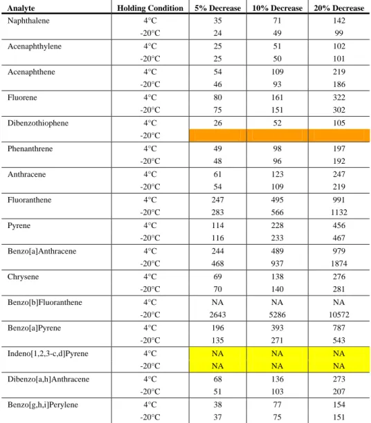
PAHs (MHT=14 days) from SQ-1 sediment ... 43 3-20 The estimated number of days until a given percentage decrease from the intercept for

PAHs (MHT=14 days) from Bedford-1 soil ... 44 3-21 Mean concentration (ng/g), coefficient of variation (CV), and significance of slope across time

for analytes with CVs>25% ... 45 3-22 Estimated number of days until a 20% decrease in concentration could be observed for

those analytes having a significant negative slope, an overall CV>25%, and observations greater than 2*MDL... 46 3-23 Mean PCB concentration (ng/g) and CV for all data across time accepted for analysis ... 57 3-24 PCB (ng/g) one-sample t-test of the null hypothesis Ho: the sample is from a population

with the mean equal to or greater than the Day 0 mean with statistical outliers removed... 60 3-25 P-values for the significance of the lack-of-fit and the slope from the linear regression and

the best fit simple linear model parameters on the natural log scale for PCBs by sediment

and holding condition ... 61 3-26 The estimated number of days until a given percentage decrease from the intercept for

PCBs (MHT=14 days) ... 62 3-27 Mean concentration (ng/g) and coefficient of variation (CV) for all pesticide data across

time accepted for analysis ... 71 3-28 Surrogates used to correct each pesticide analyte for SQ-1 sediment and Bedford-1 soil... 73 3-29 Pesticides (ng/g) one-sample t-test of the null hypothesis Ho: the sample is from a

population with the mean equal to or greater than the Day 0 mean... 75 3-30 P-values for the significance of the lack-of-fit and the slope from the linear regression

and the best fit simple linear model parameters on the natural log scale for pesticides by

sediment/soil and holding condition ... 76 3-31 The estimated number of days until a given percentage decrease from the intercept for

(13)

Table Page 3-32 Sediment/soil properties of materials used in metal acid-extraction study ... 87 3-33 Heavy metals (μg/g) one-sample t-test of the null hypothesis Ho: the sample is from a

population with the mean equal to or greater than the Day 0 mean... 87 3-34 P-values for the significance of the lack-of-fit and the slope from the linear regression

and the best fit simple linear model parameters on the natural log scale for heavy metals

for each sediment and holding condition ... 90 3-35 The estimated number of days until a given percentage decrease from the intercept for

each sediment and holding condition for heavy metals (MHT=182 days) by sediment and

(14)

(15)

List of Figures

Figure Page

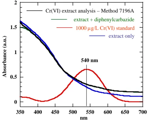
3-1 UV/Vis spectra of a) Cr(VI) 1000 mg/L standard, b) Bedford plot-6 Cr(VI) extract

solution, c) Bedford plot-6 Cr(VI) extract solution and diphenylcarbazide, and

d) Bedford plot-6 extract solution prepared as prescribed by SW-846 Method 7196A... 18

3-2 Observed Cr(VI) concentration for Soil 125A at both the 4°C and -20°C holding

temperature over holding time and associated Day 0 nonparametric bounds; there was not a significant trend through time ... 21

3-3 Observed Cr(VI) concentration for Soil 126D at both the 4°C and -20°C holding

3-4 Observed Cr(VI) concentration for Soil 123 at both the 4°C and -20°C holding

temperature over holding time, associated Day 0 nonparametric bounds, and the

significant decreasing trend for sediment held at 4°C... 23

3-5 Observed Cr(VI) concentration for Soil 125B at both the 4°C and -20°C holding

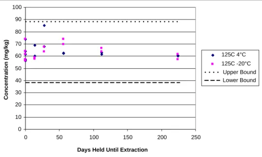
3-6 Observed Cr(VI) concentration for Soil 125C at both the 4°C and -20°C holding

3-7 Cr(VI) extract concentration stored at room temperature or 4°C as a function of time for

the Frontier Hard Chrome site sandy soil... 26

3-8 Cr(VI) extract concentration stored at room temperature or 4°C as a function of time for

the Boomsnub soil at depths of 0.5, 3.0 or 5.5 feet ... 27

3-9 Observed acenaphthylene concentration for Eagle Harbor soil at both the 4°C and -20°C

holding temperature by holding time, significant regression lines, and associated Day 0

nonparametric bounds (2*MDL is indicated by the red line)... 47

3-10 Observed fluorene concentration for Eagle Harbor soil at both the 4°C and -20°C

holding temperature by holding time, significant regression line, and associated Day 0

nonparametric bounds ... 47

3-11 Observed phenanthrene concentration for Eagle Harbor soil at both the 4°C and -20°C

3-12 Observed pyrene concentration for Eagle Harbor soil at both the 4°C and -20°C holding

temperature by holding time and associated Day 0 nonparametric bounds; there were no

(16)

Figure Page

3-13 Observed chrysene concentration for Eagle Harbor soil at both the 4°C and -20°C

3-14 Observed benzo[a]pyrene concentration for Eagle Harbor soil at both the 4°C and -20°C

3-15 Observed acenaphthylene concentration for SQ-1 sediment at both the 4°C and -20°C

holding temperature by holding time and associated Day 0 nonparametric bounds; there

was no significant trend... 50

3-16 Observed fluorene concentration for SQ-1 sediment at both the 4°C and -20°C holding

temperature by holding time and associated Day 0 nonparametric bounds; there was no

significant trend... 50

3-17 Observed phenanthrene concentration for SQ-1 sediment at both the 4°C and -20°C

3-18 Observed pyrene concentration for SQ-1 sediment at both the 4°C and -20°C holding

3-19 Observed chrysene concentration for SQ-1 sediment at both the 4°C and -20°C holding

3-20 Observed benzo[a]pyrene concentration for SQ-1 sediment at both the 4°C and -20°C

3-21 Observed acenaphthylene concentration for Bedford-1 soil at both the 4°C and -20°C

3-22 Observed fluorene concentration for Bedford-1 soil at both the 4°C and -20°C holding

significant trend (2*MDL is indicated by the red line) ... 53

3-23 Observed phenanthrene concentration for Bedford-1 soil at both the 4°C and -20°C

3-24 Observed pyrene concentration for Bedford-1 soil at both the 4°C and -20°C holding

3-25 Observed chrysene concentration for Bedford-1 soil at both the 4°C and -20°C holding

3-26 Observed benzo[a]pyrene concentration for Bedford-1 soil at both the 4°C and -20°C

(17)

Figure Page

3-27 SQ-1 sediment raw Aroclor 1254 data and surrogate recovery as a function of holding

time (days to extraction)... 58

3-28 SQ-1 surrogate corrected data as a function of the age of extract... 58

3-29 Observed Aroclor 1254 concentration for SQ-1 sediment at both the 4°C and -20°C holding

3-30 Observed PCB 153 concentration for Tri-Cities soil at both the 4°C and -20°C holding

temperature by holding time, significant regression lines, and associated Day 0

3-31 Observed Aroclor 1254 concentration for Housatonic River sediment at both the 4°C and

-20°C holding temperature by holding time, significant regression lines, and associated

Day 0 nonparametric bounds... 64

3-32 Observed Aroclor 1260 concentration for Housatonic River sediment at both the 4°C and

3-33 Observed Aroclor 1242 concentration for Tri-Cities soil at both the 4°C and -20°C holding

3-34 Observed Aroclor 1260 concentration for Tri-Cities soil at both the 4°C and -20°C holding

significant negative trend ... 67

3-41 SQ-1 sediment raw "-chlordane data and surrogate recovery ... 72

(18)

Figure Page

3-43 Bedford-1 soil raw 4,4’-DDD data and surrogate percent recovery ... 74

3-44 Observed 4,4’-DDD concentration for Housatonic River sediment at both the 4°C and

-20°C holding temperature by holding time and associated Day 0 nonparametric bounds; there was no significant trend... 79

3-45 Observed 4,4’-DDE concentration for Housatonic River sediment at both the 4°C and

3-46 Observed 2,4’-DDT concentration for Housatonic River sediment at both the 4°C and

-20°C holding temperature by holding time, significant regression line, and associated

3-47 Observed 4,4’-DDT concentration for Housatonic River sediment at both the 4°C and

-20°C holding temperature by holding time and associated Day 0 nonparametric bounds; there was no significant trend... 80

3-48 Observed "-chlordane concentration for SQ-1 sediment (surrogate corrected) at both the

4°C and -20°C holding temperature by holding time and associated Day 0 nonparametric bounds; there was no significant negative trend ... 81

3-49 Observed trans nonachlor concentration for SQ-1 sediment (surrogate corrected) at both

the 4°C and -20°C holding temperature by holding time and associated Day 0

nonparametric bounds; there was no significant trend ... 81

3-50 Observed 4,4’-DDE concentration for SQ-1 sediment (surrogate corrected) at both the

4°C and -20°C holding temperature by holding time and associated Day 0 nonparametric bounds; there was no significant negative trend ... 82

3-51 Observed 4,4’-DDD concentration for SQ-1 sediment (surrogate corrected) at both the

4°C and -20°C holding temperature by holding time and associated Day 0 nonparametric bounds; there was no significant trend ... 82

3-52 Observed 2,4’-DDT concentration for SQ-1 sediment (surrogate corrected) at both the

3-53 Observed "-chlordane concentration for Tri-Cities soil at both the 4°C and -20°C holding

3-54 Observed (-chlordane concentration for Tri-Cities soil at both the 4°C and -20°C holding

3-55 Observed trans nonachlor concentration for Tri-Cities soil at both the 4°C and -20°C

was no significant negative trend ... 85

3-56 Observed 4,4’-DDD concentration for Bedford-1 soil (surrogate corrected) at both the

4°C and -20°C holding temperature by holding time, significant regression lines, and

(19)

Figure Page

3-57 Observed 4,4’-DDT concentration for Bedford-1 soil (surrogate corrected) at both the

3-58 Observed As concentration for Sinclair River sediment for both the wet and dry holding

condition over holding time and associated Day 0 nonparametric bounds ... 89

3-59 Observed Zn concentration for Sinclair River sediment for both the wet and dry holding

3-60 Observed Pb concentration for Sinclair River sediment for both the wet and dry holding

3-61 Observed As concentration for Wilmington soil for both the wet and dry holding

3-62 Observed Cu concentration for Sinclair River sediment for both the wet and dry holding

3-63 Observed Cu concentration for Wilmington soil for both the wet and dry holding

3-64 Observed Pb concentration for Wilmington soil for both the wet and dry holding

3-65 Observed Zn concentration for Wilmington soil for both the wet and dry holding

(20)

(21)

Acknowledgements

The authors wish to thank all those individuals whose cooperation and participation contributed to the development of the research data and this report. We greatly appreciate the guidance, assistance, and technical review provided by the Task Order Project Officer Dr. Brian Schumacher of the U.S. Environmental Protection Agency, National Exposure Research

Laboratory (NERL), Las Vegas, Nevada. Also, for their technical reviews of the draft report, we thank Mr. Gary Robertson and Mr. John Zimmerman of Human Exposure and Atmospheric Sciences Division and Environmental Sciences Division, respectively, US EPA, NERL, Las Vegas, NV. We also wish to acknowledge Robert Maxfield and Joe Blazevich of US EPA Regions 1 and 10, respectively, as the original Regional Methods Initiative requesters, which lead to this project.

We are grateful to J. Gareth Pearson, Director of the Technical Support Center at Environmental Sciences Division, US EPA, NERL, Las Vegas, NV, for his original call for potential

soil/sediment materials identification. We wish to thank the following individuals for their time and effort in identification and collection of the soil/sediment materials utilized in this study: Joe Blazevich (retired), Hahn Gold (formerly) and Gerald Dodo, US EPA, Region 10; Young Chang, US EPA Region 2; Larry Heinis and Dave Mount, US EPA, Duluth, MN; Byron Mah, Robert Maxfield, Cornell Rosiu, Dan Granz, Carolyn Casey, Mike Nalipinski, and Kymberlee Keckler, US EPA, Region 1; Marilyn Jupp, and William Sargent, US EPA, Region 5; Ken Mallory, Debbie Colquitt, and Archie Lee, US EPA, Region 4; and Frank Van Ryn, Koch Industries.

(22)

(23)

Section 1 Introduction

Extraction and determination of a contaminant concentration (organic and metal) in soil, water, sediment, and other matrices is vital to estimating their impact on the environment. In an attempt to standardize the determination of contaminant levels in various matrices, the U.S.

Environmental Protection Agency (USEPA) has established a set of procedures, protocols, and techniques for sampling, preservation, and analysis for various matrices and contaminants: the USEPA SW-846 Test Methods for Evaluating Solid Wastes, Physical/Chemical Methods (USEPA, 2000). As part of sample handling protocols, maximum holding times (MHT) have been established to protect sample integrity and provide sufficient time for analyses. Holding times have been defined as the length of time an environmental media (e.g., water, soil, sediment, etc.) can be stored (under specific conditions) after collection and prior to analysis with reasonable assurance that the analyte of interest’s concentration does not change

significantly (Bayne et al., 1993).

Depending upon the matrix, analyte in question, and analytical methodology, soil/sediment sample MHTs vary (Table 1-1). Extraction and analysis of contaminants beyond MHTs may cause significant problems; for instance, analyses may be “flagged” or designated as estimates, often requiring expensive resampling and analysis.

Holding times and preservation requirements are set to assure that contaminant concentrations do not change significantly between sampling and extraction because of intrinsic biogeochemical reactions, such as biotic and abiotic degradation, volatilization, oxidation/reduction, or

irreversible sorption. The fate of contaminants in soils and sediments have been extensively studied and reported in the literature. With the exception of hexavalent Cr (and other redox sensitive metals) and volatile organic compounds (VOCs); however, only a limited number of studies have looked at the impact of holding times and preservation techniques on the

determination of contaminant concentration in soils and sediments.

1.1 Chromate [Cr(VI)]

Chromium has been utilized in various products and manufacturing processes throughout the world and chromium containing wastes have been discharged to the environment (Petura et al., 1998). The two common valance states of chromium [Cr(III) and Cr(VI)] exhibit vastly different physical/chemical behavior and toxicological properties. Hexavalent Cr is fairly soluble in aqueous environments compared to the insoluble and immobile trivalent Cr, and it is more toxic to exposed organisms (Petura et al., 1998). Hence, there has been considerable research focusing on development of a valance sensitive extraction technique for soils, sediments, and solid wastes (USEPA, 1983, 1986).

In 1986, SW-846 Method 3060 was removed as a regulatory approved method for extraction of Cr(VI) in solid samples primarily due to instability of the extract. Chromate determinations have

(24)

been shown to be effected by oxidation/reduction reactions resulting from sample treatment: i.e., drying (Bartlett and James, 1996; James, 1994; James and Bartlett, 1983); base dissolution of Fe(II) bearing minerals and subsequent reduction of Cr(VI) (Qafoku et al., 2003); and induction of, or maintenance of anaerobic conditions (Vitale et al., 1997a). Fendorf (2000), in a recent

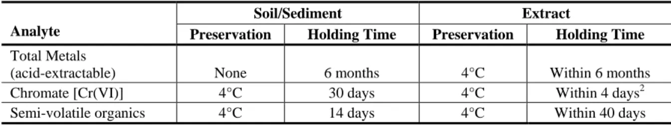
Table 1-1. Soil/sediment sample preservation, and holding times, and extract preservation, and holding times1.

Soil/Sediment Extract

Analyte _{Preservation Holding}_{Time Preservation Holding}_Time

Total Metals

(acid-extractable) None 6 months 4°C Within 6 months Chromate [Cr(VI)] 4°C 30 days 4°C Within 4 days2 Semi-volatile organics 4°C 14 days 4°C Within 40 days 1 _{From Tables 3-1 and 4-7 of the SW-846 manual (USEPA, 2000).}

2 _{From Table 4-7 of SW-846 manual, but values of 3 days, 24 hrs, and as soon as possible are also quoted in Cr(VI) extraction method} (3060A) and Cr(VI) detection methods (e.g., Methods 7196A, and 7199).

review of Cr(VI) reduction, concluded that biological processes are the principal means by which Cr(VI) is converted to Cr(III) in aerobic systems. In addition, he surmised that the aeration status of a system is of primary dependence, while pH and concentrations of reduced phases appeared to be secondary. A modified Cr(VI) extraction method (Method 3060A; US EPA, 2000) was adopted after extensive study of a large set (>1500) of diverse field samples ranging from anoxic sediments to chromite ore processing residue (Table 1-2) (Vitale at al., 1994; 1997ab; 2000; James 1994; James et al., 1995).

Table 1-2. Changes made in Method 3060.1

Change in Extraction Protocol Method 3060 Method 3060A

Wet sample wt. (g) 100 2.5 Alkaline digest solution volume (mL) 400 50 Solution to solid ratio 4 20 Digestion temperature (°C) Near boiling 90 – 95 Digestion time (min) 30 – 45 60 Nitric acid acidification pH 7 - 8

pH 7 – 8, but if <7, discard and start over 1_{After Vitale et al., 1994.}

SW-846 Method 3060A delineates a MHT of 30-d prior to extraction. Vitale et al. (2000)

performed one of the few studies designed to specifically investigate the effect of sample holding time on Cr(VI) extraction from contaminated solid matrices. They utilized soils contaminated with low, medium, and high levels of chromite ore processing residue (COPR) to follow Cr(VI) extraction (Method 3060A) concentration as a function of time (up to 30 days) from collection to extraction. The relative percent difference (RPD) between holding times of 1-d to 30-d for low, medium, and highly contaminated COPR soils were 7.4, 0.5, and 1.8%, respectively. Given that

(25)

an RPD of >20% has been suggested as the maximum allowable variation between duplicates without mandated re-extraction, the results of Vitale et al. (2000) clearly demonstrated Cr(VI) stability in the COPR soils for at least 30 days when stored at 4°C.

Chromate analysis of solid matrix extracts may be analyzed by a number of methods (USEPA, 2000). Common methods of Cr(VI) detection are SW-846 Methods 7196A or 7199, which utilize the reaction of Cr(VI) with diphenylcarbizide (DPC) to produce a red-violet complex whose absorbance may be measured spectrophotometrically at 540 nm. The MHT for Cr(VI) extracts prior to analysis ranges from “as soon as possible” to 3 days (see footnote of Table 1-1) depending on the method of analysis. The 24-h MHT associated with Method 7196A probably arises from the prescribed (40 CFR, Part 136) holding time for aqueous Cr(VI) samples. Vitale et al. (2000); however, investigated the Cr(VI) extract (Method 3060A/7196A) stability over a 7-d period. They concluded that for the COPR soils investigated Cr(VI) extract stability over the 7-d

period was acceptable when extracts were stored in the dark at 4oC.

1.2 Semi-Volatile Organic Compounds

Reactions of pesticides and other semi-volatile organic compounds (SVOCs) in the soil environment have been reviewed in great detail (Sawhney and Brown, 1989; Cheng, 1990 for example). Of primary concern is that most organic compound concentrations will be reduced with time as a result of biotic and abiotic reactions. Even at 4°C, most of these degradation processes continue, albeit at a slower rate. For certain contaminants in a soil matrix; however, the abiotic and biotic reactions are of limited concern up to and well beyond the MHT. For instance, in a recent study of organochlorine pesticides in archived (air-dried) sludge-amended United Kingdom (UK) soils, half-lives of 8 pesticides ranged from 7 to 25 years (Meijer et al., 2001). The authors suggested that volatilization was the major process causing pesticide concentration depletion since microbial activity is typically minimal in air-dried soils. While these soils were air-dried and stored in sealed containers (unlike samples to be analyzed under SW-846), the reported half-lives are substantial and gives one pause regarding a 14 day until extraction, 4°C MHT for pesticides as specified in SW-846.

In a recent study of selected polychlorinated biphenyls (PCBs) and polyaromatic hydrocarbons (PAHs) in UK field soils (protected against leaching), slight increases in PCBs (congeners 28, 101, or 158) studied were observed (Cousins and Jones, 1998). The concentration increases were attributed to gas phase deposition. Smith et al. (1976) and Moein (1976) studied an Aroclor 1254 spill site over a two-year time frame and observed no significant reduction. For studied PAHs, the lighter molecular weight (MW) species (acenaphthene and phenanthrene) exhibited

statistically significant losses, while heavier MW species [fluoranthrene, and

benzo(ghi)perylene] showed no loss over a 281 day period. In sludge-amended soils, half-lives for naphthalene and benzo(ghi)perylene varied from 2.1 years to 9.1 years, respectively (Wild et al., 1990; 1991).

A more recent study of historically contaminated soils investigated the impact of cold storage on PAH extraction concentrations (Rost et al., 2002). Soil samples from two different sites exhibited very different results. Quantitative recovery of PAHs from soil stored at 4°C in the dark was observed throughout an 8 to 10 month holding time. Under identical storage conditions, a soil

(26)

from a railroad sleeper preservation site exhibited significant losses of PAHs with low MW compounds being more affected than the higher MW compounds. After only a 2 week holding

time, ≤ 3-ring PAH concentrations had decreased by 29% to 73%; lesser but still significant

losses of up to 5-ring PAHs were also observed. Rost et al. (2002) demonstrated that PAH loss was due to aerobic microbial metabolism as PAH loss was not observed in soil treated with sodium azide prior to storage. In addition, stabilization against PAH loss was achieved by storing the soil at -20oC.

1.3 Acid Extractable Heavy Metals

Acid digestion of solid matrices (e.g., soils, sediments) for the determination of heavy (trace) metals concentrations is not a total digestion technique. According to SW-846 Method 3050B, the extraction is designed to dissolve almost all elements that could become “environmentally available”. For non-redox sensitive trace metals (Cd, Cu, Pb, Zn, etc.), a hot acid extract will probably be little affected in a time frame of years, which is reflective of the 6 month MHT prior to extraction. The aforementioned heavy metal contaminants are retained in soils by processes (e.g., ion exchange, specific adsorption, precipitation etc.) that are extractable to the same extent over long periods of time. The extraction method allows the sample to be dried, but drying is not required; however, sample homogeneity is typically more easily achieved with dried and sieved materials.

1.4 Objectives

The overall objective of this research effort was to investigate the stability of selected contaminants in soil/sediment samples as a function of holding time prior to extraction and analysis. Contaminants of interest centered on SVOCs, particularly PAHs, PCBs, and pesticides, Cr(VI), and several heavy metals. Contaminant specific objectives were:

1. Determine if selected SVOC contaminant concentrations in soil/sediment changed with time

when held in storage beyond their established extraction MHTs under current preservation

techniques and at -20oC;

2. Determine if Cr(VI) concentrations change when held in storage beyond their established

MHTs under current preservation techniques and at -20oC;

3. Determine if extracted Cr(VI) concentrations change when held beyond the analysis MHT

(24-h) when held in the dark at room temperature (~ 20oC) or 4°C;

4. Determine if air-drying soil samples will adversely impact hot acid extractable metal

concentrations;

5. Determine if hot acid extractable metal concentrations change when samples are held beyond

(27)

Section 2 Materials and Methods

2.1 Soils/Sediments Identification, Collection and Selection

A total of 19 soils/sediments were collected for this study (Table 2-1). Except for the Sinclair Inlet and SQ-1 sediment, samples of soils/sediments were obtained from contaminated sites throughout the United States. The Sinclair Inlet sample was obtained from an ongoing study at the Battelle Marine Sciences Laboratory and the SQ-1 sediment was obtained from J. Blazevich (retired), USEPA Region 10, Manchester, WA.

The SQ-1 sample was a sediment sample collected from Sequim Bay, WA in 1986, an area relatively free of contamination by PAH, PCBs, and chlorinated pesticides. The grain size and carbon content was similar to that of contaminated sediment in urban areas around the Puget Sound. Originally the sediment was placed in a cement mixer, spiked with a mixture of organic chemicals, mixed 7 hours, subsampled for chemical analysis, bottled in 2-oz glass jars with

Teflon lined lids, and stored frozen at -20oC. The results for the post-mixing chemical analyses

indicated this reference material was homogenous (coefficient of variation, CVs, usually less than 20%) and the recovery of the analytes was usually greater than 50% of the expected concentration. Over a period of 10 years, between 1986 and 1996, several laboratories analyzed between 20 to 80 jars of SQ-1 and recovered about 50% of the expected concentrations of most of the analytes. The CVs for the mean of these results were about 50%.

Sediment samples were drained of excess water by vacuum filtration. Samples of each material were semi-quantitatively screened for contaminant type and concentration. From the 19

soil/sediment samples identified, 12 materials were utilized during the course of the project (Table 2-1; material in bold). Selection of materials for use was based on contaminants present, their concentration, and the amount of material. For instance, the CIC New Jersey sample was rejected for heavy metal study because only a single contaminant, arsenic, was present in significant quantity, and after screening the quantity of <2 mm material was insufficient for the study.

2.2 Experimental Design

The overall objective of this project is to provide scientific data on contaminant concentration changes through time. The expected contaminant concentration changes through time should be generally linear and potentially, curvilinear. Regression analysis allows the estimation of an equation relating contaminant concentration as a function of time. Regression analysis with replication provides greater power in testing for a particular response (e.g., a linear relationship) than does the equivalent design analyzed with an analysis of variance (ANOVA). The increased power for testing in the regression is directly related to the increased number of degrees of freedom for the error term. For example, for six analysis time points with two replicates at each time and a linear response, Table 2-2 shows that there are only six degrees of freedom for testing

(28)

the linear (or curvilinear) response with an ANOVA compared to ten degrees of freedom (nine if a quadratic term is needed) in the regression analysis. Regression analysis, on the other hand, specifically tests for a consistent change through time (either linear or curvilinear).

Table 2-1. Available soils/sediments.

Sample Sample type Suspected contaminants

1 Housatonic River Freshwater sediment PCBs/Pesticides 2 Tri-Cities NY2 Soil PCBs/Pesticides

3 Eagle Harbor Soil PAHs

4 SQ-1 Marine sediment PAHs/PCBs/Pesticides

5 Bedford-1 Soil PAH

6 Bedford plot-6 Soil Cr(VI) 7 Frontier Hard Chrome Site-2 Soil Cr(VI) 8 Boomsnub site-0.5’ Soil Cr(VI) 9 Boomsnub site-3.0’ Soil Cr(VI) 10 Boomsnub site-5.5’ Soil Cr(VI) 11 Stratford, CT Army engine plant Soil Cr(VI) 12 Sinclair Inlet, WA Marine sediment SVOCs/Metals 13 Wilmington, NC Soil PAHs/Metals 14 Eastland Woolen Mills, ME Soil DDT, DDE, Dieldrin 15 Richland site-1 Soil Several Pesticides 16 Frontier Hard Chrome Site-1 Soil Cr(VI)

17 EPA-Athens Soil Cr(VI)

18 EPA-Athens Soil Cl-Pesticides 19 CIC New Jersey Soil Metals

Table 2-2. Comparison of analysis of variance and regression assuming six time points for chemical analysis, two replicate analyses at each time, and a linear relationship.

Analysis of Variance Regression Analysis

Sources of Variation Degrees of Freedom Sources of Variation Degrees of Freedom

Mean 1 Mean 1

Times (t) (t-1) = 5 Slope = b1 1

Lineara 1 Remainderb t*r - 2 = 10

Remainder 4 Lack of Fitc 4

Within Timesb t*(r-1) = 6 True Error t*(r-1) = 6 Total t*r = 12 Total t*r = 12 a_{The indented sources of variation represent the splitting of the main source of variation (not indented) listed above.} b

Error for testing the null hypothesis that the slope equals zero.

c _{The sum of the degrees of freedom from the split sources of variation equal the degrees of freedom for the main source of} variation listed above.

Regression analysis has the added advantage of being able to estimate a spline point where the relationship may change abruptly.

(29)

2.2.1 Soils/Sediments Homogenization, Analysis, Storage and Extraction Schedule

An experimental design based on regression analysis was constructed. The design consisted of

initial (T = 0) extraction and analysis of multiple subsamples (4 SVOCs; 5 CrO4, and metals),

which were followed by extraction and analysis of four subsamples (two per storage technique; see below) at multiples of the analyte’s MHT.

The selected soils/sediments were hand-screened (< 2mm) to remove rocks and twigs. The 12 sediment/soil samples were homogenized by hand through repeated cone and quartering and recompositing the sieved material. Materials were then subsampled (cone and quartered) for characterization of water content, total organic carbon content (by combustion; Nelson and Sommers 1996), particle size analysis (hydrometer method; Gee and Bauder 1986), and pH determined from a 1:1 soil:water mixture with a combination glass electrode (Thomas, 1996). The selected soils/sediments were hand cone and quartered to obtain T = 0 samples. Initial (T = 0) sample extraction and analysis was performed on 4 (SVOCs) or 5 [Cr(VI) and metals] subsamples of a given sediment/soil. After subsampling for T = 0 samples, remaining materials were cone and quartered until a given subsample mass, at least 12 times the mass required for a given extraction, was obtained. This material was quartered and each quartered subsample placed in either a glass jar with Teflon-lined lid (SVOCs extraction) or polycarbonate centrifuge tubes

(CrO4 and metals) and stored under specific conditions (depending on contaminant type). This

procedure was performed repeatedly until four subsamples for each holding time were obtained (the number of MHT elements depended on the contaminant(s) under study). The storage conditions and sampling times were as follows:

• The chromate holding time study utilized soil/sediment numbers 6-11 (Table 2-1). Twelve

samples of each soil/sediment were stored at 4°C and 12 samples at -20°C. For each holding

time, two containers (duplicates) were analyzed for each holding condition (4°C and -20°C).

Specifically, the MHT multiples were 0, 0.5*MHT, MHT, 2*MHT, 4*MHT, and 8*MHT. These MHT multiples were equivalent to 0, 14, 28, 56, 112, and 224 days, respectively.

• In addition to following the stability of CrO4 as a function holding time prior to extraction, the

stability of the CrO4 extract concentration was followed with time. At T = 0, the CrO4

concentration was determined in the initial 5 extracts within 24 hrs of extraction. The remaining extract solutions, standards, laboratory blanks, and matrix spikes were placed in brown glass bottles and stored room temperature. Another 5 subsamples were extracted (with a

new set of standards, laboratory blanks, and matrix spikes), and the T = 0 CrO4 concentration

in each extract determined. This second set of extract solutions, standards, laboratory blanks, and matrix spikes were placed in brown glass bottles and stored at 4°C. The Cr(VI) extracts were analyzed at 1, 3, 7, 14, 28, and 56 days. Extracts from sediment/soil numbers 7-10 were utilized for this study (Table 2-1).

The SVOC holding time study utilized soil/sediment numbers 1-5 (Table 2-1). Twelve samples

of each soil/sediment were stored at 4°C and 12 samples were stored at -20°C. For each

(30)

-20°C). Specifically, the MHT multiples were 0, 0.5*MHT, MHT, 2*MHT, 3*MHT, 6*MHT, and 12*MHT. These MHT multiples were equivalent to 0, 7, 14, 28, 42, 84, and 168 days, respectively.

• The Sinclair Inlet sediment and the Wilmington, NC soil were used to study the stability of As,

Cu, Pb, and Zn as a function of holding time and solid material drying treatment (soil/sediment

numbers12 and 13 in Table 2-1). Eight samples were stored at 4°C and 8 samples were

air-dried for 5 days, crushed, sieved (<2 mm) and stored at room temperature. Duplicate samples

of the material stored at 4°C and air-dried samples were extracted and analyzed at multiples of

the MHT (0, 0.5*MHT, MHT, 1.5*MHT, and 2*MHT); equivalent to 0, 90, 183, 284, and 392 days.

2.2.2 Cr(VI) Extraction and Analysis

Chromate extraction of all soils/sediments was performed strictly according to SW-846 Method 3060A-Alkaline Digestion for Hexavalent Chromium. Analysis of the sediment/soil extracts was conducted according SW-846 Method 7196A-Chromium, Hexavalent (colorimetric). The

colorimetric procedure was performed as prescribed except that in the interests of waste

minimization the colorimetric solutions (analyte solutions, standards, laboratory standards, and QA solutions) were produced in 10 mL volumes rather than the suggested 100 mL volume. Colorimetric determinations were performed using a Perkin-Elmer Lambda 19 dual beam spectrophotometer. QA reviewed data tables are provided in Appendix A.

2.2.3 SVOC Extraction

Housatonic River; Tri-Cities, NY; Eagle Harbor; SQ-1; and Bedford-1 soils/sediments were extracted using SW-846 Method 3540C-Soxhlet Extraction, a procedure for extracting

nonvolatile and semivolatile organic compounds from solids. A deviation from this method was implemented for samples SQ-1 and Bedford-1 because the high moisture content of these

samples caused incomplete extraction using the Method 3540C-Soxhlet Extraction. A thumbnail sketch of the procedure and the deviations are noted below for each of the soils/sediments.

Housatonic River, Eagle Harbor, and Tri Cities — Ten g of sample was mixed with 10 g

anhydrous Na2SO4ina 125 mL Qorpak jar, 100 mL of methylene chloride was added; and the jar

rolled on a modified rock tumbler for 2 h. This mixture was transferred to a Soxhlet thimble and

put into the Soxhlet extractor. The jar was rinsed three times with 50 mL methylene chloride and the rinsate added to the thimble. The soil/sediment was extracted overnight with 350 mL

methylene chloride. The following day, the extract was evaporated using a Kuderna-Danish apparatus to <25 mL. The solvent exchanged to hexane, transferred to a 25 mL volumetric flask, and brought to volume using hexane. Activated copper was added to 1 mL (Housatonic River and Tri-Cities) or 2 mL (Eagle Harbor) of the resultant solution to remove the sulfur interference as described in SW-846 Method 3660B-Sulfur Cleanup Method. Deviations to SW-846 Method 3660B were:

• 0.2 mL of the copper treated Housatonic River extract or 0.05 mL Tri-Cities extract was

placed on a conditioned Florisil column and eluted with 9 mL of 1:9 acetone:hexane mixture as described in SW-846 Method 3620-Florisil Cleanup. The eluate was evaporated to 1.0 mL

(31)

• 1.0 mL of the copper treated Eagle Harbor extract was placed on a silica column as described in SW-846 Method 3630C-Silica Gel Cleanup. The column was pre-eluted with 40 mL pentane and the pentane discarded. One mL of sample was added to the column and eluted with 25 mL pentane. This fraction was then discarded. 25 mL of 2:3 methylene

chloride:pentane solution was added to the column and this fraction was collected in a Qorpak jar. The solution was then transferred to the Kuderna-Danish evaporator, solvent exchanged to

cyclohexane, evaporated to 1.0 mL, and 100 μL of internal standard PP-1195 was added.

SQ-1 — Initially, a 15 g sample was mixed with 10 g anhydrous Na2SO4and 10 g activated

copperin a 125 mL Qorpak jar. One hundred mL of methylene chloride was added to the jar and

the jar rolled on a modified rock tumbler for 2 h. With the exception of the initial step, the SQ-1

sediment followed the protocol used for Housatonic River, Eagle Harbor and Tri Cities soils/sediments.

Bedford-1 — Due to limited amount of soil, 5 to 6 g of soil was utilized for each subsample. The mass of soil was placed in 250 ml Qorpak jars. Prior to extraction, 0.5 g of sample was removed from the jars to determine percent dry weight. One hundred mL of methylene chloride,

10 g activated copper and 50 g anhydrous Na2SO4 wereadded. The vessel was shaken vigorously

then put on a modified rock tumbler for two hours to homogenize the components. The

suspension was transferred to a Soxhlet thimble and put into the Soxhlet extractor. The jar was rinsed three times with 50 mL methylene chloride and the rinsate added to the thimble. The soil was extracted overnight with 350 mL methylene chloride. The following day the sample was evaporated using a Kuderna-Danish apparatus to 25 mL, solvent exchanged to hexane, and again treated with activated copper as described in SW-846 Method 3660B-Sulfur Cleanup. 0.5 mL of the extract was placed on the Florisil column as described in SW-846 Method 3620-Florisil Cleanup and 0.5 mL was placed on the silica column as described in SW-846 Method 3630C-Silica Gel Cleanup. Both eluates were evaporated using a Kuderna-Danish apparatus to 1.0 mL, solvent exchanged to cyclohexane, and 0.1 mL of laboratory produced internal standard was added.

2.2.4 SVOC Analysis

All SVOC extracts were analyzed prior to the SVOC 40 day MHT. Polyaromatic hydrocarbon analysis of the SVOC extracts followed SW-846 Method 8270C-Gas Chromatography/Mass Spectrometry (GC/MS) with specifications and modifications as noted. PAHs were separated via high resolution capillary gas chromatography and identified and quantified using electron impact mass spectrometry. A data system interfaced to the GC/MS was used to control acquisition and to store, retrieve, and manipulate mass spectral data. The PAHs listed in Table 2-3 were

identified and measured in selected ion monitoring mode (SIM). Tuning followed the parameters from the instrument manufacturer, which uses a compound PFTBA that is bled into the

instrument. Inertness of the system was assessed using linearity and calibration check compounds (CCCs). The only deviation from SW-846 protocol was for sensitivity and compound degradation, which was addressed via other system checks, not specifically by a system performance check compound (SPCC). QA reviewed data tables and QA narratives are provided in the Appendix A.

(32)

Table 2-3. PAH Analyte List

Analyte Quantitation Ion Confirmation Ion

Naphthalene 128 127

Acenaphthylene 152 153

Acenaphthene 154 153

Fluorene 166 165

Dibenzothiophene 184 139

Phenanthrene 178 176

Anthracene 178 176

Fluoranthene 202 101

Pyrene 202 101

Benzo[a]anthracene 228 226

Chrysene 228 226

Benzo[b]fluoranthene 252 253 Benzo[k]fluoranthene 252 253

Benzo[e]pyrene 252 253

Benzo[a]pyrene 252 253

Perylene 252 253

Indeno[1,2,3-c,d]pyrene 276 277

Dibenzo[a,h]anthracene 278 279

Benzo[g,h,i]perylene 276 277

Surrogate Standards Quantitation Ion Confirmation Ion

Naphthalene-d8 136 137

Acenaphthene-d10 164 162

Phenanthrene-d10 188 184

Chrysene-d12 240 236

Perylene-d12 264 265

Internal Standards Quantitation Ion Confirmation Ion

Acenaphthylene-d8 160 161

Pyrene-d10 212 106

(33)

Table 2-4. PCB (Aroclors and Congeners) and chlorinated pesticide analyte list. PCBs - Aroclors

Aroclor 1242 (or 1016) Aroclor 1248

Aroclor 1254 Aroclor 1260

PCB - Congeners

CB Numbera CAS Nomenclatureb CAS Registry Numberc 8 2,4'-dichlorobiphenyl 34883-43-7

18 2,2',5-trichlorobiphenyl 37680-65-2 28 2,4,4'-trichlorobiphenyl 7012-37-5 29 2,4,5-trichlorobiphenyl 15862-07-4 44 2,3',3,5'-tetrachlorobiphenyl 41464-29-5 49 2,2',4,5'-tetrachlorobiphenyl 41464-40-8 50 2,2' 4,6=-tetrachlorobiphenyl 62796-65-8 52 2,2',5,5'-tetrachlorobiphenyl 35693-99-3 66 2,3'.4,4'-tetrachlorobiphenyl 32598-10-0 87 2,2' 3,4,5'-pentachlorobiphenyl 38380-02-8 101 2,2',4,5,5'-pentachlorobiphenyl 37680-73-2 104 2,2',4,6,6'-pentachlorobiphenyl 56558-16-8 105 2,3,3',4,4'-pentachlorobiphenyl 32598-14-4 118 2,3',4,4',5-pentachlorobiphenyl 31508-00-6 126 3,3',4,4',5-pentachlorobiphenyl 57465-28-8 128 2,2',3,3',4,4'-hexachlorobiphenyl 38380-07-3 138 2,2' 3,4,4',5'-hexachlorobiphenyl 35065-28-2 153 2,2',4,4',5,5'-hexachlorobiphenyl 35065-27-1 154 2,2',4,4',5,6'-hexachlorobiphenyl 60145-22-4 170 2,2',3,3',4,4',5-heptachlorobiphenyl 35065-30-6 180 2,2',3,4,4',5,5'-heptachlorobiphenyl 35065-29-3 183 2,2',3,4,4',5',6-heptachlorobiphenyl 52663-69-1 184 2,2',3,4,4, 6,6'-heptachlorobiphenyl 74472-48-3 187 2,2',3,4',5,5',6-heptachlorobiphenyl 52663-68-0

188 2,2' 3,4' 5,6,6'-heptachlorobiphenyl 74487-85-7 195 2,2',3,3',4,4',5,6-octachlorobiphenyl 52663-78-2 200c 2,2',3,3',4,5',6,6'-octachlorobiphenyl 40186-71-8 206 2,2'3,3',4,4',5,5',6-nonachlorobiphenyl 40186-72-9 209 2,2'3,3',4,4',5,5',6,6'-decachlorobiphenyl 2051-24-3

a_{Ballschmiter and Zell numbering scheme.}

b_{Chemical Abstracts, Tenth Collective Index, Index Guide, American Chemical Society, Columbus, Ohio, 1982.} c_{CB 200 in the Ballschmiter and Zell numbering scheme.}

(34)

Table 2-4, Continued

Chlorinated Pesticides

Aldrin

alpha-BHC

beta-BHC

gamma-BHC (Lindane)

delta-BHC

4,4'-DDE 4,4'-DDD 4,4'-DDT (cis) alpha-Chlordane

(trans) gamma-Chlordane Tech. Chlordane

Dieldrin Endosulfan I

Endosulfan II

Endrin Endrin Aldehyde

Endrin Ketone

Heptachlor Heptachlor Epoxide

Toxaphene Endosulfan Sulfate

Hexachlorobenzene

2,4'-DDD 2,4'-DDE 2,4'-DDT Mirex trans-Nonachlor

Surrogate Standards

PCB 103 PCB 198

Internal Standards

Tetrachloro-m-xylene (TCMX) Octachloronaphthalene (OCN) Hexabromobiphenyl (HBB)

Analysis of chlorinated pesticides followed SW-846 Method 8081A. Analysis of polychlorinated biphenyls (PCBs) as Aroclors or individual congeners followed SW-846 Method 8082. Both

analyses utilized capillary gas chromatography with 63Ni electron-capture detection. The internal

(35)

and linear condition but if outside data quality objectives (DQOs), the analytical run was allowed to complete and then assessed with surrogates and spike recoveries. QA Reviewed data tables and QA narratives are provided in the appendix. Table 2-4 lists the PCBs and pesticides targeted. 2.2.5 Metal Digestion (Acid-Leachable) and Analysis

The Wilmington soil and Sinclair Inlet sediment samples were digested using the acid-leachable digestion detailed in SW-846 Method 3051-Microwave Assisted Acid Digestion of Sediments, Sludges, Soils, and Oils. Digestates were analyzed via SW-846 Method 6020-Inductively Coupled Plasma-Mass Spectrometry. The method measures ions produced by a radio-frequency inductively coupled plasma. Analyte species originating in a liquid are nebulized and the

resulting aerosol transported by argon gas into the plasma torch. The ions produced are entrained in the plasma gas and introduced, by means of an interface, into a mass spectrometer. The ions produced in the plasma are sorted according to their mass-to-charge ratios and quantified with a channel electron multiplier. There were no deviations from the aforementioned protocols. QA reviewed data tables and QA narratives are provided in the Appendix A.

2.3 Statistical Analysis

Descriptive statistics including the mean, standard deviation, minimum, maximum, median, and

data quartiles (first quartile, Q1, equals the 25th percentile and the third quartile, Q3, equals the

75th percentile) were calculated for each sampling period and holding condition. The mean,

standard deviation, and CV (equal to the standard deviation divided by the mean) were also calculated for all data collected for a given holding condition.

Overall CVs of less than 20% for CrO4 and metals, and 25% for SVOCs suggest that data has

remained within the data quality acceptance criteria for replicate precision (Table 2-5). Even though trends may be statistically detected in such data, it would be suspect due to the normal analytical error that can be observed in chemical analysis. For analytes measured within this level of noise, one would suggest that the concentration did not decrease more than would be allowed between replicate measurements over the entire time period tested. For these analytes, estimation of a holding time from this experiment could be considered impractical.

A one-sample, one sided, t-test of the null hypothesis Ho: the data are samples from a population with a mean equal to or greater than the mean of the Day 0 concentration versus the alternative

H1: the samples are from a population with a mean less than the mean of the Day 0

concentration, was conducted to provide a measure of relevance (chemical importance) of the potential change. Simple linear regression of concentration against time was used to test 1) the null hypothesis that the slope of the natural logarithm of the concentration of each contaminant was equal to zero and 2) the null hypothesis that slopes associated with curvature (the lack-of-fit to the simple linear model) were equal to zero. Plots were used to compare the observed

concentration to the nonparametric upper and lower boundaries of the Day 0 concentration calculated as Q3+ 1.5(Q3-Q1) and Q1-1.5(Q3-Q1), respectively. The fitted regression line was included in data plots if the slope was negative and statistically different from zero.

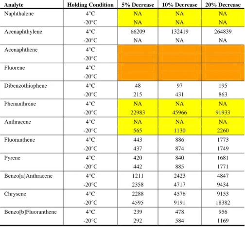
The holding time (HT), defined as the number of days until a 5%, 10% and 20% decrease in the

(36)

based on the lower 95% confidence limit of the slope estimate (βLCL). Thus, holding time for a

given percentage change (Δ%) was defined as HT = -Δ%*C0/βLCL. Using the lower 95%

confidence limit of the linear slope provides some conservatism to the holding time estimation because as the data increasingly deviate from a simple linear response, the confidence interval

increases and the slope used for estimation becomes steeper. When the estimated βLCL was

greater than 0, the concentration was estimated to be increasing instead of decreasing and the number of days until a given percentage lost was not applicable (NA). All of the analytes tested were assumed to only decrease over time since none of the analytes measured were considered a degradation product.

Chemical concentrations tend to be log normally distributed. Thus, analysis was conducted on the natural logarithm of the concentration to satisfy assumptions of the statistical analyses. Further, the natural logarithm of the concentration was used instead of the raw data scale because sediments have varying amounts (i.e., 50 to 800 mg/kg) of a given analyte. The natural log transformation rescales the observations to minimize the magnitude of the difference between the Day 0 value and the value obtained at a given percentage change. A percentage change (i.e., 10%) from a large number (say 800) has a larger magnitude difference (800-720=80) than the same percentage change from a small number (50-45=5). Thus, on the raw data scale, analytes with the same slope associated with the decrease in concentration over time but different intercepts would produce quite different estimates of the holding time. The natural log transformation reduces this effect (i.e., ln[800]-.9*ln[800]=0.67 compared to

ln[50]-.9*ln[50]=0.39). The resulting holding times would still be different; however, the magnitude of the difference would be much less than that achieved on the raw scale.

Observations were removed from data analysis including plots if they were potentially

contaminated (flagged with a B) or rejected for QC/QA reasons (flagged with an r). Analysis was conducted with and without observations considered extreme outliers, defined as Q3 + 3*(Q3-Q1) where the quartiles are derived from the Day 0 data. Extremely high outliers have a large influence on the estimated slope and, thus, the resulting holding time. Outliers in the Day 0 data were removed from analysis and plots if the within replicate CV was greater than 25%.

Observations were removed from the Day 0 data only if a single value was extreme and if that value was the furthest absolute distance from the median value. Extreme outliers observed during all other sampling times were removed from the analysis only if they made up less than 10% of the total number of observations.

Residual plots were used to assess the lack of homogeneity of variance, lack-of-fit to the linear model, potential outliers, and observations that could have exaggerated influence on the

estimated slopes. Residuals, defined as the observed minus the fitted result, are assumed to have a mean of zero and a constant variance. Residuals plotted against time should display a random pattern about zero with a constant variance across the x-axis. A consistent U-shaped pattern of the residuals would indicate the need for curvature in the model if a significant (p < 0.05) lack-of-fit was detected. The need for a spline or nonlinear model could also be indicated by a

significant lack-of-fit. However, if the concentration decreased and then increased over time, the lack-of-fit was considered analytical noise. In these cases, the simple linear model was used for the holding time estimation. A single observation that has a large amount of influence on the estimated slopes would be indicated by a residual close to zero and far away on the x-axis from