CLUSTER ENSEMBLE METHODS FOR SINGLE CELL RNA-SEQ DATA AND
DECONVOLUTION OF BULK HI-C DATA
Ruth Huh
A dissertation submitted to the faculty of the University of North Carolina at Chapel Hill in
partial fulfillment of the requirements for the degree of Doctor of Philosophy in the Department
of Biostatistics in the Gillings School of Global Public Health.
Chapel Hill
2019
Approved by:
Yun Li
Yuchao Jiang
Michael Love
Jin Szatkiewicz
Kirk Wilhelmsen
©
2019
Ruth Huh
ABSTRACT
Ruth Huh : Cluster Ensemble Methods for Single Cell RNA-Seq Data and Deconvolution of Bulk
Hi-C Data
(Under the direction of Yun Li)
Clustering single-cell RNA-seq (scRNA-seq) data is a critically important task to shed
light on tissue complexity including the number of cell types present and transcriptomic
signa-tures of each cell type. Due to its importance, several novel methods have been developed
re-cently for clustering scRNA-seq data. However, different approaches generate varying estimates
regarding number of clusters and cluster assignments making it hard to gauge which method to
use.
In the first paper, we present SAFE-clustering, Single-cell Aggregated (From
Ensem-ble) clustering, a flexible, accurate and robust method for clustering scRNA-seq data.
SAFE-clustering takes results from multiple SAFE-clustering methods to build one consensus SAFE-clustering. In
our current implementation, individual solutions are ensembled using three hypergraph-based
partitioning algorithms, namely hypergraph partitioning algorithm (HGPA), meta-cluster
algo-rithm (MCLA) and cluster-based similarity partitioning algoalgo-rithm (CSPA). In our evaluations,
SAFE-clustering generates high-quality clustering, in terms of both cluster number and cluster
assignment, across various datasets.
In the second paper, we present SAME-clustering, Single-cell Aggregated Clustering via
Mixture Model Ensemble, where we follow a similar pipeline with SAFE-clustering but change
the ensemble clustering method to a probabilistic framework. Specifically, SAME-clustering uses
a finite mixture model of multinomial distributions. Results show that our SAME-clustering
ensemble method, using a mixture model, yields enhanced clustering, in terms of both cluster
assignments and number of clusters.
In the third paper, we shift gears from analyzing scRNA-seq data to C data.
which measures spatial interactions important in providing information for gene regulation and
3D structure of the genome. Standard Hi-C data are generated from millions of cells, thus
pro-viding a population average measure of heterogeneous cells. Therefore, observed differences in
contact information are confounded by relative proportions of cell types among samples. It is
important to adjust for these proportions in downstream bulk Hi-C analysis. To date, there are
no deconvolution methods applied to Hi-C data to estimate these proportions. We propose using
nonnegative matrix factorization (NMF) for a matrix decomposition-based framework to estimate
ACKNOWLEDGEMENTS
I would like to thank my advisor Professor Yun Li, for taking me as her student later
in my PhD career. I am grateful for her guidance in my disseratation and support of my
well-being throughout my 3 years working with her. I would also like to thank all of my committee
members, Professor Yuchao Jiang, Professor Michael Love, Professor Jin Szatkiewicz, Professor
Kirk Wilhelmsen, and Professor Di Wu, for your helpful input and questions on my dissertation
topic.
I would like to thank all Li lab members. You have helped me with programming in
many platforms, widening my biological and statistical knowledge, and improving my
presen-tation skills. I would like to especially thank Yuchen Yang for collaborating closely with me
throughout my dissertation.
I am thankful for all the support and encouragement I received from my friends and
family. I am grateful for my mom and in-laws who took care of my daughter during my studies,
my daughter Yena for giving me joy in the midst of my studies and my husband Hojoon for
per-severing with me through various life stages. Last but not least, I would like to thank my Father
TABLE OF CONTENTS
LIST OF TABLES . . . .
ix
LIST OF FIGURES . . . .
x
CHAPTER 1: LITERATURE REVIEW . . . .
1
1.1
Motivation behind first and second papers . . . .
1
1.2
Some Recent Clustering Methods for single-cell RNA-seq . . . .
3
1.3
Ensemble Methods and their advantages . . . .
7
1.4
Motivation for third paper . . . .
9
1.5
Deconvolution methods for RNA-seq . . . 10
CHAPTER 2: SAFE-clustering: Single-cell Aggregated (From Ensemble) Clustering
for Single-cell RNA-seq Data . . . 14
2.1
Overview of SAFE-clustering . . . 14
2.2
Expression matrix normalization . . . 15
2.3
Benchmarking Datasets . . . 15
2.4
Improving and running four state-of-the-art methods . . . 16
2.5
Hypergraph Partitioning Cluster Ensemble Algorithms . . . 22
2.6
Performance evaluation using ANMI . . . 24
2.7
Benchmarking of three hypergraph partitioning algorithms in SAFE . . . 25
2.8
Results . . . 28
2.9
Discussion . . . 35
CHAPTER 3: SAME-clustering: Single-cell Aggregated Clustering via Mixture Model
Ensemble . . . 37
3.2
Expression matrix normalization . . . 38
3.3
Benchmark Datasets . . . 39
3.4
Implementation and Evaluation of Individual clustering methods . . . 39
3.5
SAME-clustering method using the multinomial mixture model . . . 50
3.6
Diversity of individual cluster results to improve SAME-clustering . . . 58
3.7
Results . . . 61
3.8
Discussion . . . 69
CHAPTER 4: Reference free Hi-C Deconvolution . . . 70
4.1
Overview of Hi-C Deconvolution using NMF . . . 71
4.2
Simulation of Bulk Samples . . . 71
4.3
NMF method . . . 72
4.4
Preliminary Results . . . 74
4.5
Selecting Significant Features . . . 81
4.6
Results . . . 87
4.7
Discussion . . . 94
LIST OF TABLES
Table 1
Characteristics of the 12 benchmarking datasets . . . 16
Table 2
Additional characteristics of the 12 benchmarking datasets . . . 28
Table 3
Major characteristics of 15 benchmarking datasets . . . 39
Table 4
Evaluating effect of gene filter on SC3 . . . 40
Table 5
Evaluating robustness of Seurat and SAME across number of PCs used . . . 42
Table 6
Evaluating ADPclust centroid detection . . . 45
Table 7
Assessing the effect of gene filtering on individual methods . . . 49
Table 8
Difference in ARIs with and without gene filtering . . . 50
Table 9
Evaluation of NMF and CIBERSORT deconvolution . . . 78
Table 10
Evaluation different feature selection methods . . . 82
Table 11
Results implementing the 2-step NMF . . . 88
LIST OF FIGURES
Figure 1
Overview of SAFE-clustering . . . 15
Figure 2
PCA plot to determine number of clusters . . . 18
Figure 3
Seurat performace evaluation . . . 19
Figure 4
t-SNE+kmeans performance evaluation . . . 21
Figure 5
Comparing HGPA, MCLA, and CSPA . . . 27
Figure 6
Diversity among individual clustering methods . . . 29
Figure 7
Benchmarking of SAFE-clustering in 12 published datasets . . . 30
Figure 8
Accuracy evaluation of the inferred number of cluster . . . 31
Figure 9
Evaluating robustness of t-SNE+kmeans . . . 32
Figure 10
Evaluating robustness of SAFE-clustering . . . 34
Figure 11
Overview of SAME-clustering . . . 38
Figure 12
Visualization to determine number of clusters . . . 41
Figure 13
Elbow plot to determine number of PCs to be used . . . 43
Figure 14
t-SNE+kmeans clusters from automatically determined centers . . . 46
Figure 15
t-SNE+kmeans clusters from manually selected centers . . . 47
Figure 16
Performance of AIC and BIC for model selectiong . . . 56
Figure 17
Determining iterations needed for EM algorithm . . . 57
Figure 18
Pairwise similarities of individual methods for Zeisel dataset . . . 59
Figure 19
Evaluating SAME-clustering with all or a diverse set of individual results . . . 60
Figure 20
Evaluation of SAME-clustering on 15 benchmark datasets . . . 62
Figure 21
Similarity between estimated and true clusters . . . 64
Figure 22
Similarity between estimated and true clusters (adjusted) . . . 65
Figure 23
SAME-clustering determines limitations in true annotations . . . 66
Figure 24
NK marker gene expression in the novel cluster . . . 67
Figure 25
SAME-clustering discovers a novel cluster . . . 68
Figure 27
Difference of Top Fano Factor bins between HAP1 and HeLa cells . . . 76
Figure 28
Plot of True vs Estimated cell type proportions for HAP1 and HeLa . . . 79
Figure 29
Plot of Estimated cell type contacts against Simulated cell type contacts . . . 80
Figure 30
Observed contacts vs the fitted contacts . . . 80
Figure 31
Relationship between feature score and fold change . . . 83
Figure 32
Relationship between feature score and difference . . . 84
Figure 33
Signature bins for HAP1 and HeLA cells . . . 86
Figure 34
PCA and PC2 loadings plot separating HAP1 and HeLa cells . . . 88
Figure 35
Estimated proportions from 2-step NMF . . . 89
Figure 36
Correlation of estimated and simulated interchromosomal expression . . . 89
Figure 37
Correlation of Observed vs Fitted contacts . . . 90
Figure 38
PCA and PC2 loadings plot separating Patski and MEF cells . . . 91
Figure 39
Difference of Hi-C contacts between Patski and MEF cells . . . 92
CHAPTER 1: LITERATURE REVIEW
1.1
Motivation behind first and second papers
The development RNA-sequencing (RNA-seq) has allowed us to obtain a global view
of the transcriptome in different species and cell types (Wang et al., 2009). Cells from different
cell types have unique transcriptomes, informative of their roles in and contribution to normal
cellular function, cell fate determination, early development, as well as disease development
(Bi-ase et al., 2014; Deng et al., 2014; Goolam et al., 2016; Yan et al., 2013; Huang, 2009; Tang et al.,
2011; Liu and Trapnell, 2016). Moreover, even among cells of the same cell type, gene expression
levels are found to be highly variable (Buganim et al., 2012; Guo et al., 2010; Hashimshony et al.,
2012; Shalek et al., 2013). Because of such heterogeneity among cells, the commonly adopted
bulk RNA-seq measurements may obscure and mask true behaviors of distinct cell types
(Trap-nell et al., 2014). Therefore, transcriptomic analysis should be carried out at a single cell level
(Tang et al., 2011).
Single cell RNA-seq (scRNA-seq) analysis led to, among others, the identification of
existing and novel cell types, characterization of cells, prediction of cell fate, classification of
tumor subpopulations and investigation of cellular heterogeneity (Treutlein et al., 2014; Li et al.,
2016; Xin et al., 2016; Arsenio et al., 2014; Gr¨
un et al., 2015; Patel et al., 2014; Min et al., 2015;
Wills and Mead, 2015; Baron et al., 2016; Biase et al., 2014; Darmanis et al., 2015; Deng et al.,
2014; Goolam et al., 2016; Li et al., 2017; Ting et al., 2014; Yan et al., 2013; Zeisel et al., 2015;
Zheng et al., 2017). For all these applications, single cell clustering is a crucial preprocessing
step. After clustering the single cells, all of the following analyses can be conveniently carried out:
identification and examination of cell type specific gene expression signatures (Rozenblatt-Rosen
et al., 2017; Yan et al., 2013), cell type covariate adjustment for differential expression analysis
(Li et al., 2017; Gr¨
un et al., 2015), and deconvolution of bulk RNA expression data (Baron et al.,
Due to its importance, it is not surprising to find many existing single cell RNA-seq
clustering methods. The high dimensionality of scRNA-Seq data pose a grand challenge for
un-supervised cell clustering (Xu and Su, 2015; Lin et al., 2017; Wang et al., 2017). Principal
com-ponent analysis (PCA) and t-Distributed Stochastic Neighbor Embedding algorithm (t-SNE)
(Maaten and Hinton, 2008) are both commonly used for data visualization and dimensional
re-duction prior to single-cell clustering. The dimension reduced data is often followed by kmeans
to perform the actual clustering (Shin et al., 2015; Kiselev et al., 2017). Other recent methods
include RaceID (Gr¨
un et al., 2015), RCA (Li et al., 2017), SC3 (Kiselev et al., 2017), Seurat
(Satija et al., 2015), CIDR (Lin et al., 2017), DIMM-SC (Sun et al., 2017), and SIMLR (Wang
et al., 2017). Different clustering methods manipulate the input scRNA-seq data differently, for
example, by using different distance metrics and dimensionality reduction methods. Therefore,
clustering results may have inconsistencies due to methods taking different approaches and/or
making different underlying assumptions. As a matter of fact, cluster results from different
meth-ods are found to be rather dissimilar, with discrepancies occurring both in the estimated number
of clusters and in actual single-cell-level cluster assignment. Therefore the use of two or more
clustering methods is recommended for more accurate and comprehensive overview of cell
cluster-ing (Freytag et al., 2017). However, when true cluster labels are unknown, it would be difficult
to select the best method, prior to or even after clustering analysis (even with multiple methods
implemented separately).
Since it is hard to select the optimal method when true cell types are unknown,
ensem-bling information from multiple individual methods becomes an appealing alternative. cluster
en-semble solutions are known to provide robust and improved quality solutions (Strehl and Ghosh,
2002; Ghosh and Acharya, 2011) in many other contexts including analysis of cell signalling
dy-namics and protein folding (Hubner et al., 2005; Kuepfer et al., 2007). Ensemble solutions range
from probabilistic approaches to graph partitioning methods (Ghosh and Acharya, 2011). In
addition to providing robust and improved cluster results, cluster ensemble methods provides a
way to estimate an optimal number of clusters, which is important when there are dramatically
1.2
Some Recent Clustering Methods for single-cell RNA-seq
There are many clustering methods developed specifically for single-cell RNA-seq data.
Some like RaceID (Gr¨
un et al., 2015) and GiniClust (Jiang et al., 2016) are tailored for rare cell
type identification. Most other methods focus on identification of common cell types. Desirable
features of scRNA-seq clustering methods include dimension reduction, gene filtering,
normal-ization and detection of number of clusters. The following methods have some or all of these
features in their pipelines.
SC3
SC3 (Kiselev et al., 2017), consensus clustering of scRNA-seq data, includes several
steps in their clustering methods. It can take different types of inputs, ranging from Reads
Per Kilobase per Million mapped reads (RPKM), Fragments Per Kilobase per Million mapped
reads (FPKM), Transcripts Per Million mapped reads (TPM), Counts Per Million mapped reads
(CPM), and counts, where counts are converted to CPM to account for sequencing depth. The
normalized expression matrix is log-transformed after adding ones to avoid taking log of zeros.
SC3, then filters out genes/transcripts that are expressed in less than 10% of cells or more than
90% of cells to remove rare and ubiquitous genes/transcripts. 10% is the default value that can
be adjusted by the user and this gene filtering step is optional as an entirety. After the filtering
step, three distance metrics, Euclidian distance, Pearson and Spearman correlations, are
calcu-lated between single cells. These three distance matrices are then transformed using both PCA
and eigenvector decomposition of a Laplacian graph separately. Next, kmeans clustering is
per-formed on these transper-formed distance matrices. A consensus matrix of the different kmeans
clus-tering solutions is constructed using the cluster-based similarity partitioning algorithm (CSPA)
(Strehl and Ghosh, 2002). Lastly, this consensus matrix is clustered assuming an a priori
k
clus-ters. SC3 has a method to estimate
k
using the Tracy-Widom distribution (Tracy and Widom,
1994).
SC3 has a moderate computational cost and therefore, they employ support vector
ma-chine (SVM) (Ben-Hur, 2001) model to speed up computation for large datasets. For datasets
with more than 5,000 single cells, a subset of 5,000 single cells are randomly selected and
cells. Althogether, SC3 includes all important features of scRNA-seq clustering, which are
dimen-sion reduction using PCA and Laplacian, gene filtering of rare and ubiquitous genes,
normaliza-tion of input expression matris, and estimanormaliza-tion of number of clusters through the Tracy Widom
distribution (Tracy and Widom, 1994).
CIDR
CIDR’s (Lin et al., 2017) main advantage is that it imputes dropout genes expression
values to improve clustering results. Dropouts are common in scRNA-seq data where there is less
starting mRNA material to work with compared to bulk RNA-seq experiments and can cause
failures in amplification in the RNA-seq experiment. The type of input taken by CIDR are
log-arithmic transformed CPM values. After dropout determination and imputation, dissimilarity
matrix is calculated by using squared Euclidean distance between pairs of cells. CIDR employs
principal coordinate analysis (PCoA) for dimensional reduction. For ease, CIDR R package
au-tomatically determines the number of principal coordinates to use for dimensional reduction in
its
nPC
function. However, users may choose to alter the number of Pco’s to use by searching
for the elbow point in the plot showing proportion of variation explained by each principal
co-ordinate. With the dimension reduced dissimilarity matrix, hierarchical clustering is applied to
assign cluster labels to single cells. The number of clusters,
k
, is estimated with the
Calinski-Harabasz index (Cali´
nski and Harabasz, 1974). One key feature missing in CIDR is gene filtering,
which is most likely because it attempts to solve the problem of rarely expressed genes through
imputation.
Seurat
Seurat (Butler et al., 2018) combines dimensional reduction with graph partitioning
methods and takes as input raw Unique Molecular Identifier (UMI) counts or read counts. The
expression matrix is first filtered to exclude single cells with less than 200 expressed genes, and to
exclude genes expressed in fewer than three single cells. Thus, single cells with
<
200 expressed
genes are not given a final cluster label, resulting in missing cluster labels. For counts input,
Seurat normalizes, for each single cell, by the total gene expression in each cell and multiplies by
a scale factor of 10,000. Natural log transformation is subsequently applied after normalization.
Seurat then scales the data by removing unwanted sources of variation, by regressing out number
non-UMI data. Furthermore, Seurat can regress out batch effect, cell alignment rate, percent
of mitochondrial genes, and cell cycle. Next, PCA is performed on the scaled data to reduce
dimensionality. To cluster the cells, Seurat first constructs a K-nearest neighbor (KNN) graph
with Euclidean distance in PCA space, where edges are drawn between similar cells. These edge
weights are refined based on Jaccard distance which measures the dissimilarity between local
neighborhoods. The cells are clustered by applying modularity optimization techniques (Blondel
et al., 2008), and the number of clusters,
k
, is determined during the clustering process.
There are couple of parameters that need to be specified by the user for better results.
The resolution parameter is influential on cluster results as it sets the ’granularity’ of clustering.
Larger values lead to greater number of clusters and Seurat finds that setting this resolution
pa-rameter between 0.6-1.2 typically returns good clustering results. Another papa-rameter that needs
to be specified is the number of PCs to use in the clustering. Users can examine the plot of the
standard deviation of principal components and determine a cutoff at the elbow of the plot. This
decision can be rather arbitrary when there is not a clear elbow. Another option is to use the
embedded JackStrawPlot function in the Seurat R package, to discover significant PCs. Overall,
Seurat includes all important features of scRNA-seq clustering, however, the ambiguous decision
needed to make for the resolution parameter and the number of PCs to use, may pose a challenge
for potential users. Aside from clustering, Seurat provides many convenient downstream analysis
features including finding differentially expressed genes and t-SNE visualization.
t-SNE+kmeans
t-distributed Stochastic Neighbor Embedding (t-SNE) is a popular approach to visualize
high dimensional data in two or three dimensional space and has been used widely to visualize
single cell clusters (Gr¨
un et al., 2015; Zheng et al., 2017). It is an improvement to their previous
technique, Stochastic Neighbor Embedding (SNE) (Hinton and Roweis, 2003), as it is easier
to optimize, reduces the crowding of points towards the center, and helps with the appearance
of clusters (global structure) in a map. Briefly, high dimensional Euclidean distances between
data points are converted into joint probabilities that represent similarities. These similarities
are also computed for the low dimensional counterparts. The basic concept is that if the low
dimensional points correctly model the similarity between the high-dimensional data points,
converted into probabilities using a Gaussian distribution. In the low dimensional map, distances
are converted into probabilities using a Student t-distribution with 1 degree of freedom which
has much heavier tails than a Gaussian. Heavy tails allow for moderately dissimilar points in
high dimension to be modeled by a much larger distance in low dimensions, thus resolving the
crowding problem and giving global structure in cluster visualization. Solution is found through
minimizing a single Kullback-Leibler divergence between a joint probability distribution,
P
, in
the high- dimensional space and a joint probability distribution,
Q
, in the low-dimensional space
using the gradient descent method. One parameter that needs to be specified by the user is the
perplexity parameter. Perplexity can be seen as a measure of the effective number of neighbors
and t-SNE is reportedly fairly robust to a range of values, and typical values are between 5 and
50.
After reducing to two or three dimensional space, data can be clustered via kmeans.
The R package
Rtsne
, does an initial reduction of space using PCA, and implements the
Barnes-Hut algorithm (Van Der Maaten, 2014) to mitigate the heavy computational burden that comes
with minimizing the Kullback-Leibler divergence using gradient descent for large datasets. t-SNE
+ kmeans is lacking key features of scRNA-seq clustering, which are gene-filtering, normalization,
and determination of number of clusters. Gene-filtering and normalization can be added easily
when finalizing the gene expression matrix. However, a method needs to be developed to estimate
the number of clusters.
ADPclust(Wang and Xu, 2017) may be used as an intermediate step between t-SNE
and kmeans to determine an optimal number of clusters. ADPclust is an adaptive density peak
detection method using nonparametric multivariate kernel density estimation. To determine the
number of clusters,
k
, cluster assignments are evaluated through the silhouette index (Rousseeuw,
1987) using a grid of values for both bandwidth and number of clusters. ADPclust chooses a
plug-in bandwidth estimator that minimizes the asymptotic mean integrated squared error
(AMISE) to estimate the parameters of the multivariate kernel distribution. The cluster centroids
and number of clusters that produces the maximum average silhouette index can be carried
SIMLR
Single-cell interpretation via multikernel learning (SIMLR) (Wang et al., 2017) takes
raw gene expression matrix as input and applies a log 10 transformation prior to analysis. SIMLR
learns a similarity metric through learning proper weights for several Gaussian kernels. The
advantage of using multiple kernels lies in its flexibility in comparison to a single kernel and
therefore, can capture diverse statistical characteristics of single-cell data. Then a cell-to-cell
similarity matrix in constructed and SIMLR assumes that this matrix should be approximately
block-diagonal when clusters exist. This similarity matrix is used as input, instead of the regular
gene expression matrix, to reduce the dimension of the data using t-SNE and k-means is used for
clustering.
For large-scale version of SIMLR, k-nearest-neighbor (KNN) is used to approximate
the pairwise similarity matrix. After the similarity matrix is obtained, spectral clustering is
used instead of applying kmeans after t-SNE, because t-SNE is more computationally expensive.
SIMLR supplies two ways to estimate the optimal number of cluster: eigengap and separation
cost. They utilize eigenvalues and eigenvectors which can easily become computationally
expen-sive with larger datasets. Therefore, it is not feasible to estimate number of clusters using these
methods for large datasets. An important feature of scRNA-seq clustering that SIMLR lacks is
gene-filtering. However, SIMLR claims to address the problem of high dropouts by
implement-ing a rank constraint in the learned similarity matrix and graph diffusion which improves weak
similarity measures.
1.3
Ensemble Methods and their advantages
Cluster ensembles aim to combine the information from individual clustering methods to
provide an improved overall clustering of the given data. The advantage of cluster ensembles lies
in its robustness by providing better average clusterings across datasets and its novelty in finding
a combined solution unattainable by individual clustering methods (Topchy et al., 2005). Many
papers have found that diversity and quality of partitions influence the performance of ensemble
solutions (Fern and Lin, 2008; Fern and Brodley, 2003; Kuncheva and Hadjitodorov, 2004;
to improve ensemble results. We will now briefly lay out some graph partitioning approaches and
one probabilitic approach to cluster ensembles.
Graph partitioning methods uses a concept called hypergraph. Briefly, for the
j
th
clus-tering method, we use
v
ik
(note subscript
j
is omitted for presentation brevity) to denote the
i
th
row of the hypergraph
H
j
, which is the row vector for the cluster labels (coded as binary
dum-mies or indicator functions) of the
i
th
single cell, where
v
ik
=
1
,
the i
th
cell
∈
the k
j
thcluster
0
,
the i
th
cell /
∈
the k
j
thcluster
and
k
j
= 1
,
2
, ..., K
j
,
with
K
j
being the total number of clusters from the
j
th
clustering method.
Here, each column is a hyperedge, representing one particular cluster identified by that method.
An overall hypergraph
H
is constructed by combining individual hypergraphs (from individual
methods). Cluster-based Similarity Partitioning Algorithm (CSPA), HyperGraph-Partitioning
ALgorithm (HGPA) and Meta-Clustering Algorithm (MCLA) all use the concept of hyperedges
and hypergraphs, but they are inherently different on how they use them. Specifically, CSPA
uses the similarity matrix that is constructed from the hypergraph, where two objects are fully
similar if they are always in the same cluster, to perform partitioning. HGPA partitions the
hypergraph by cutting a minimal number of hyperedges that creates
k
clusters of approximately
equal size. This algorithm would not be optimal when cluster sizes vary a lot. MCLA collapses
related hyperedges(clusters) and assigns each cell to the most related collapsed hyperedge. This
collapsed hyperedge is referred to as a meta-cluster, thus the name Meta-Clustering Algorithm.
A probablistic approach to solve the cluster ensemble problem would be to use a
multi-nomial mixture model (Topchy et al., 2004). Assume that the number of consensus clusters is
known to be ˆ
k
, where each is indexed by ˆ
l
. For each consensus cluster ˆ
l
and each individual
method
q
, we have a multinomial distribution
β
ˆ
(
q
)
l
of dimension
k
(
q
)
, where
k
(
q
)
is the number of
clusters determined by the
q
t
h
clustering method. Each draw from this multinomial distribution
would correspond to the cluster label from the
q
t
h
individual clustering. With these probabilistic
Combining multiple clustering comes with new challenges. One is that there is no
ex-plicit correspondence between labels from different clustering methods. Another added
complex-ity is that different cluster methods may contain different number of clusters, which adds to the
correspondence problem. Both ensemble methods discussed completely avoids the label
corre-spondence problem through the use of hyperedges and multinomial distribution and is able to
deal with varying numbers of clusters determined by individual methods.
1.4
Motivation for third paper
Most tissue samples are heterogeneous consisting several cell types, and cell type
pro-portions are highly variable between samples. When transcriptional profiles of bulk RNA-seq
samples are compared among different phenotypic states, cell type composition is a strong
con-founder of observed differences (Repsilber et al., 2010; Palmer et al., 2006; Baron et al., 2016).
Transcript abundance may vary due to the physiological condition of the samples, individual
vari-ation, and relative proportions of cell types (Shen-Orr and Gaujoux, 2013). Since gene expression
varies across cell types in a tissue, these variations in each sample is better captured by reporting
differences in cell type proportions among the samples. Without relative proportions of cell
sub-sets, it is hard to distinguish whether increased gene expression is due to an overexpression of a
gene, or to merely having more cells that express that gene. Also, without accounting for varying
cell type proportions, it would be hard to identify which cell type the observed difference came
from. Failing to adjust for relative cell type proportions between samples suffers from increased
false positives of differentially expressed genes when cell type proportion difference is correlated
with the phenotype of interest, difficulty in attributing the observed difference to a specific cell
type, and restricts interpretability of results (Shen-Orr and Gaujoux, 2013).
Cellular compositions of samples have been deconvolved using Fluorescence Activated
Cell Sorting (FACS), Laser Capture Micro-dissection(LCM), and Translating Ribosome Affinity
Purification(TRAP) to separate defined cell types (Okaty et al., 2011). However, these methods
encounter technical difficulties with limited availability of surface markers, increases stress on
Shen-Orr et al., 2010; Shen-Shen-Orr and Gaujoux, 2013). Therefore, deconvolution of bulk RNA-seq gene
expression is more efficient, unbiased and economical (Qiao et al., 2012).
Hi-C is a genome-wide (”all-against-all”) variant of chromosome conformation capture
technique, which measures spatial interactions and provides information for gene regulation and
3D structure of the genome. It gives another level of information compared to RNA-seq data.
Just like RNA-seq data, Hi-C data are generated from millions of cells, providing a population
average measure of heterogeneous cells. Therefore, it has the same problem with bulk-RNA seq
data where observed differences in contact information are confounded by relative proportions
of cell types among samples. There is a vast amount of research on deconvolution methods for
RNA-seq data, but none have been applied on Hi-C data. Therefore, I study several RNA-seq
de-convolution methods that were developed to solve for cell type composition of biological samples,
to see what methods can be effectively applied to bulk Hi-C deconvolution.
1.5
Deconvolution methods for RNA-seq
Most deconvolution methods have gene expression matrix of samples and a cell type
specific expression profile as input. The goal is to solve for the cell type proportion of samples.
The gene expression matrix is a
n
×
p
matrix we denote as
X
, cell-type specific expression matrix
is a
k
×
p
matrix,
H
, and cell type proportion of samples is a
n
×
k
,
W
, matrix. The different
de-convolution methods are a variation of solving for
W
in
X
=
W H
in their respective ways. Below
I will go over the method and the advantages and disadvantages that come with the methods. I
aim to draw from the advantages of each method to apply it to Hi-C data.
CIBERSORT
CIBERSORT (Newman et al., 2015) takes as input a gene expression of a complex
tis-sue and cell-type gene signature matrix to find the cell type proportions using
ν
-support vector
regression. In creating the gene signature matrix, they are made more robust by minimizing
an inherent matrix property called the condition number. CIBERSORT then adaptive selects
genes from this signature matrix and solves the deconvolution problem. Support vector
regres-sion (SVR) fits a hyperplane to as many data points as possible within a distance
. Data points
signature matrix. These points are evaluated according to a linear
insensitive loss function and
provide a sparse solution to the regression where overfitting is minimized. SVR seeks to minimize
both the linear
insensitive loss function, and the L2-norm penalty function.
ν
-SVR is employed
since it sets both an upper bound on training errors and lower bound on support vectors. Higher
values of
ν
yield lower values of
. The current implementation of CIBERSORT runs
ν
-SVR with
a linear kernel for three values of
ν
= (0
.
25
,
0
.
5
,
0
.
75) to solve for
W
and saves the best value.
Best value is determined by lowest root mean squared error between
X
and
W
×
H
. Negative
re-gression coefficients are set to 0 and the other coefficients are normalized to sum to 1.
X
and
H
are normalized to zero mean and unit variance for better performance and run time. The major
challenge would be obtaining an accurate cell-type gene signature matrix to solve the problem
when pure cell type gene signature matrix may not be available. A key advantage of the method
is that it performs feature selection, where signature genes are selected to deconvolve the mixture
samples.
PERT
PERT (Qiao et al., 2012) aims to correct for two major limitations in deconvolution
methods. They develop a flexible deconvolution method to account for the possible presence of
new cell types and possible fluctuations between gene expressions between the reference profiles
and the constituent profiles. PERT compares four models. Non-negative least squares model,
N N LS
, uses linear regression framework to estimate the proportion of celltypes in each sample
and assumes that all reference profile and constituent profile are similar and require cell type
spe-cific signature genes. Non-negative maximum likelihood model,
N N M L
, makes the same
assump-tion as NNLS but uses a Latent Dirichlet Allocaassump-tion (LDA) framework. The LDA framework
uses a multinomial noise model which better fits noise in gene expression data. Non-negative
maximum likelihood model new population,
N N M L
np
, is a version of ISOLATE (Quon and
Morris, 2009), based on an LDA framework and assumes that there is an additional constituent
population in the heterogeneous sample that is not represented in the reference profile. This is
their attempt at addressing the possibility of a new cell type. PERT, a perturbation model, is
based on the
N N M L
framework and considers transcriptional variations between reference and
constituent profiles.
N N M L
is less sensitive to selection on cell type signature genes and can be
PERT takes as input reference and constituent profiles to output cell type proportions in each
sample. PERT relaxes the assumption that the provided reference distributions are a good
repre-sentation of the constituent cell populations. It introduces a multiplicative factor
ρ
g
to account
for systematic changes in gene expression, which are assumed to be equal across cell types.
DSA
Digital Sorting Algorithm, DSA (Zhong et al., 2013), takes gene expression matrix of
heterogenous samples and marker genes of cell types to solve for cell type frequencies and cell
type specific gene expression profile. DSA first estimates cell type frequencies from marker genes
by solving a system of linear equations. This step can be skipped if cell type frequencies are
already known. It then deconvolves gene expression profile of mixed tissue sample into cell-type
specific expression profiles by using the cell type frequencies that are either estimated or provided
and uses quadratic programming to solve the equation.
Quadratic programming is a Non-negative Matrix Factorization(NMF) based method
and a major drawback is the non-uniqueness of the factorization (Donoho and Stodden, 2004).
Therefore, DSA uses a set of marker genes, a gene that is only expressed in one cell type, which
is equivalent to the separability assumption for the uniqueness of NMF (Donoho and Stodden,
2004). In practice, marker genes are unknown, and this is a challenging factor for their method.
Unified statistical framework for single cell and bulk RNA sequencing data
This framework (Zhu et al., 2018) uses both scRNA-seq and bulk RNA-seq data to solve
the deconvolution problem. Single-cell RNA-seq data give a high-resolution view of cell types
that cannot been seen in bulk data. However, it has a lot of technical noise leading to many
dropout genes not seen in bulk data. For scRNA-seq data, it is important to distinguish between
genes that are truly unexpressed and genes that are missed by technical noise. This model uses
strengths from both data types, obtains estimates for cell type specific gene expression profiles,
and infers dropout gene expression and cell type proportions in bulk samples. Their inputs are
scRNA-seq, bulk-RNA seq measurements, and number of clusters, and therefore is a reference
free method. Single cell RNA-seq and bulk RNA-seq data are linked through the cell type
spe-cific gene expression profile matrix. They use single cell RNA-seq and bulk RNA-seq
simultane-ously to impute dropouts in single cell RNA-seq data and to infer the cell type mixing proportion
specific profile matrix and gibbs sampling is used to infer the probability of drop out and mixing
CHAPTER 2: SAFE-clustering: Single-cell Aggregated (From Ensemble) Clustering for
Single-cell RNA-seq Data
To date, there is no published cluster ensemble approach across multiple types of
clus-tering methods specifically designed for scRNA-Seq data. To bridge the gap, we have developed
SAFE-clustering, Single-cell Aggregated (From Ensemble) clustering, to provide more stable,
robust and accurate clustering for scRNA-Seq data. In the current implementation,
SAFE-clustering first performs independent SAFE-clustering using four state-of-the-art methods, SC3, CIDR,
Seurat and t-SNE + k-means, and then combines the four individual solutions into one
consoli-dated solution using one of three hypergraph partitioning algorithms: hypergraph partitioning
algorithm (HGPA), meta-clustering algorithm (MCLA) and cluster-based similarity partitioning
algorithm (CSPA) (Strehl and Ghosh, 2002).
2.1
Overview of SAFE-clustering
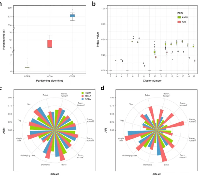
Our SAFE-clustering leverages hypergraph partitioning methods to ensemble results
from multiple individual clustering methods. The current SAFE-clustering implementation
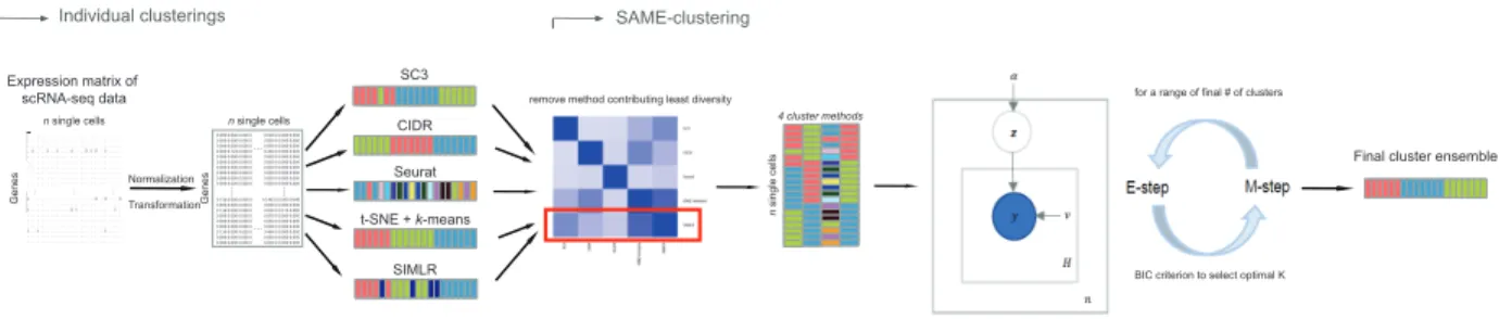
em-beds four clustering methods: SC3, Seurat, t-SNE + k-means, and CIDR. Figure 1 shows the
Figure 1: Overview of SAFE-clustering. Log-transformed expression matrix of scRNA-Seq data
are first clustered using four state-of-the-art methods, SC3, CIDR, Seurat and t-SNE + k-means;
and then individual solutions are combined using one of the three hypergraph-based partitioning
algorithms: hypergraph partitioning algorithm (HGPA), meta-cluster algorithm (MCLA) and
cluster-based similarity partitioning algorithm (CSPA) to produce consensus clustering.
2.2
Expression matrix normalization
SAFE-clustering takes an expression matrix as input, where each column represents
one single cell and each row corresponds to one gene or transcript. To make the data well-suited
for all four individual clustering methods, UMI counts are converted into Counts Per Million
mapped reads (CPM). For CIDR input, Fragments/Reads Per Kilobase per Million mapped
reads (FPKM/RPKM) data are converted into Transcripts Per Million (TPM). Lastly, for SC3,
CIDR, and t-SNE + k-means, the input expression matrix is log-transformed after adding ones
(to avoid taking log of zeros).
2.3
Benchmarking Datasets
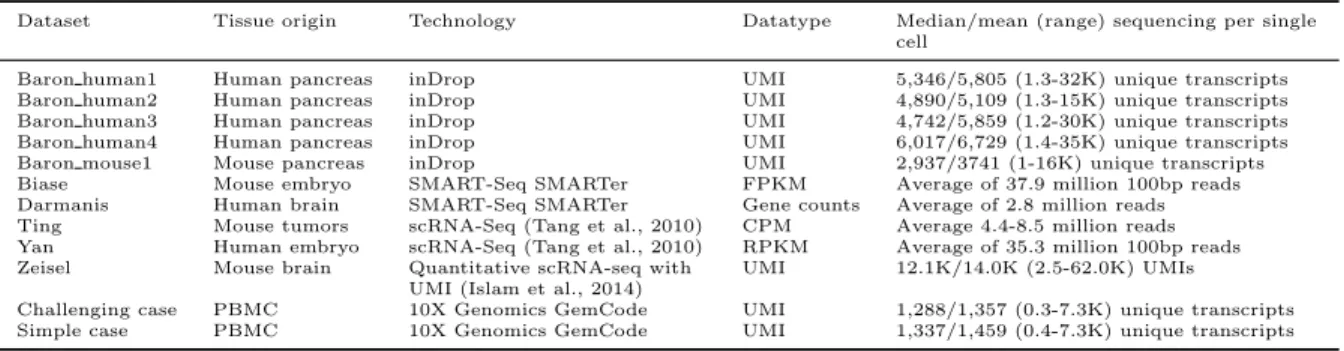
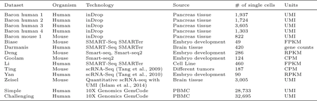
For performance evaluation, we carried out clustering analysis on 12 benchmark
scRNA-Seq datasets (Table 1) (Baron et al., 2016; Biase et al., 2014; Darmanis et al., 2015; Ting et al.,
2014; Yan et al., 2013; Zeisel et al., 2015; Zheng et al., 2017), using our SAFE-clustering and the
four individual clustering methods. All these datasets have pre-defined gold/silver-standard (we
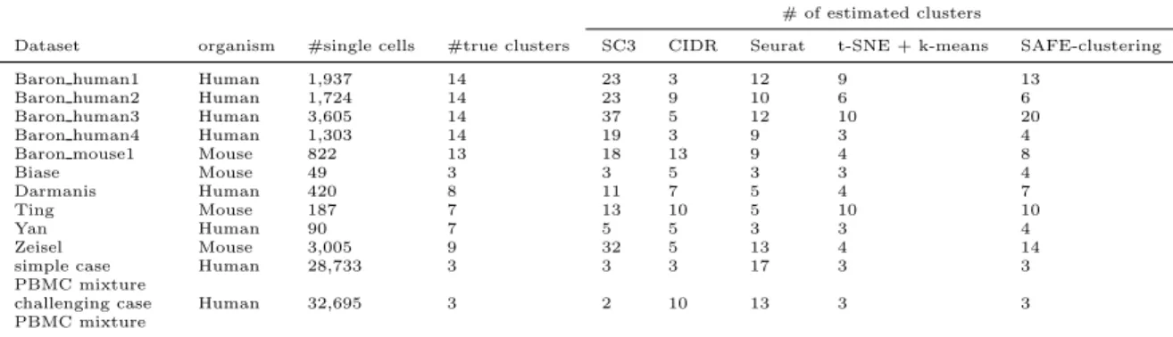
# of estimated clusters
Dataset organism #single cells #true clusters SC3 CIDR Seurat t-SNE + k-means SAFE-clustering Baron human1 Human 1,937 14 23 3 12 9 13
Baron human2 Human 1,724 14 23 9 10 6 6 Baron human3 Human 3,605 14 37 5 12 10 20 Baron human4 Human 1,303 14 19 3 9 3 4
Baron mouse1 Mouse 822 13 18 13 9 4 8
Biase Mouse 49 3 3 5 3 3 4
Darmanis Human 420 8 11 7 5 4 7
Ting Mouse 187 7 13 10 5 10 10
Yan Human 90 7 5 5 3 3 4
Zeisel Mouse 3,005 9 32 5 13 4 14
simple case PBMC mixture
Human 28,733 3 3 3 17 3 3
challenging case PBMC mixture
Human 32,695 3 2 10 13 3 3
Table 1: Major characteristics of the 12 benchmarking datasets, including organism origin,
num-ber of single cells, the numnum-bers of true and estimated clusters by SAFE-clustering and four
indi-vidual methods
Performance is measured by the similarity between the estimated cluster labels
L
E
and
the true cluster labels
L
T
using the Adjusted Rand Index (ARI) (Hubert and Arabie, 1985):
ARI
(
L
E
, L
T
) =
P
e,t
n
et2
−
[
P
e
n
e2
P
t
n
t2
]
/
n
2
1
2
[
P
e
n
e2
+
P
t
n
t2
]
−
[
P
e
n
e2
P
t
n
t2
]
/
n
2
where
n
is the total number of single cells;
n
e
and
n
t
are the number of single cells in estimated
cluster
e
and in true cluster
t
, respectively; and
n
et
is the number of single cells shared by
esti-mated cluster
e
and true cluster
t
. ARI takes a maximum value of 1 when two clustering fully
agree and its expected value is 0 when they are random clusters.
2.4
Improving and running four state-of-the-art methods
We took care in choosing the four individual clustering methods, SC3 (Kiselev et al.,
2017), CIDR (Lin et al., 2017), Seurat (Butler et al., 2018), and t-SNE+kmeans (Maaten and
Hinton, 2008), as diverse clustering methods are known to optimize ensemble solutions. These
methods also estimate the number of clusters and does not rely on apriori knowledge of the
num-ber of clusters. Furthermore, we evaluate the performance of parameters in individual clustering
methods, such as Seurat and t-SNE, and set default parameters to optimize performance of
clus-tering methods and minimize the number of parameters the users need to input. Altogether, we
created a user-friendly package, where minumum input is needed from users to create robust
SC3
Quality control (QC) metrics are calculated on the input expression matrix to detect
potentially problematic genes and/or single cells. In order to speed up computation, we first
use the Tracy-Widom method (Tracy and Widom, 1994) to estimate the number of clusters,
de-noted by ˆ
k
opt
−
SC
3
. With the estimated ˆ
k
opt
−
SC
3
, matrices of Euclidean, Pearson and Spearman
(dis)similarity metrics are calculated among single cells, followed by k-means clustering. Based
on k-means results across the three different (dis)similarity matrices and two different
dimen-sion reduction methods, a consensus matrix is computed using CSPA, followed by a hierarchical
clustering to assign the single cells into ˆ
k
opt
−
SC
3
clusters.
For the two PBMC mixture datasets (both with
>
5,000 single cells), via SC3 default
implementation, support vector machine (SVM) is employed to further speed up computation.
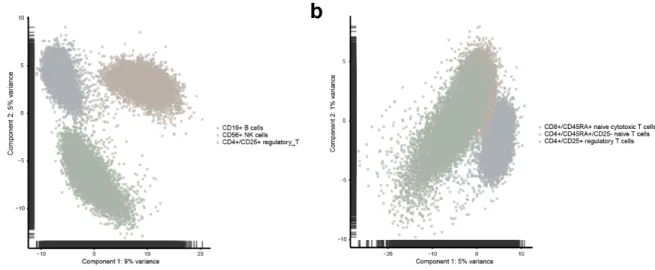
SC3 estimated 588 and 586 clusters for the simple and challenging case, respectively,
dramati-cally deviating from the truth (
k
= 3 for both two datasets). The
k
estimation method in SC3
has not been benchmarked and validated for large, shallowly sequenced datasets, and it is likely
that the distribution of eigenvalues of the covariance matrix does not adhere to the assumed
Tracy-Widom distribution (Tracy and Widom, 1994). However, clustering results of SC3 are not
affected by this since
k
estimation in SC3 is completely independent of the clustering algorithm.
Therefore, we produced a PCA plot visualization (using plotPCA function of scater R-package)
to narrow down a reasonable range of k. PCA plot suggested 3 distinct clusters for the simple
case and 2 clusters for the challenging case (Figure 2). We therefore decided, for SC3, on
k
= 3
for the simple case and
k
= 2 for the challenging case. SC3 ARI for the simple case at our
se-lected
k
= 3 is 0.995 and for the challenging case at
k
= 2 is 0.595.
CIDR
Given the normalized expression matrix, dropout candidates are identified and implicitly
imputed to mitigate the impact of lowly expressed genes. Then, dissimilarity matrix (Euclidean
distance) is calculated between single cells using the imputed data (Lin et al., 2017). As CIDR
performs principal coordinate analysis (PCoA) to reduce dimensionality, the number of principal
coordinates (PCo’s) identified, representing the estimated data dimensionality, heavily influences
the final clustering results. Here, the number of PCo’s is determined by the internal
nPC
Figure 2: PCA plot for the simple case (a) and challenging case (b) to estimate the number of
clusters to input for SC3.
into ˆ
k
opt
−
CIDR
clusters, with ˆ
k
opt
−
CIDR
estimated using the Calinski-Harabasz Index (Cali´
nski
and Harabasz, 1974).
Seurat
Seurat embeds an unsupervised clustering algorithm, combining dimension reduction
with graph-based partitioning methods. After gene and cell filtering, for counts input, Seurat
normalizes, for each single cell, by the total expression and multiplies by a scale factor of 10,000.
Natural log transformation is subsequently applied after normalization. We skip the
normaliza-tion step and only apply log transformanormaliza-tion if input data are already normalized. After that,
undesired sources of variations are regressed out. Single cells with
<
200 expressed genes would
be considered as ”NA” in the final Seurat clustering results. Data dimensionality is reduced via
principal component analysis (PCA) with the number principal components (PCs) selected by
the nPC function in the CIDR package. Graph-based clustering is carried out using the smart
local moving algorithm (SLM) (Waltman and Van Eck, 2013).
Seurat provides a ”resolution” parameter to alter the granularity of the clustering results.
However, the default ”resolution” (= 0.8) tends to result in no clustering for small datasets, as
shown in the SC3 paper (Kiselev et al., 2017). To further evaluate the performance of Seurat
on small datasets, we generated 100 subsets of samples from the Darmanis dataset, using
strati-fied random sampling without replacement where each cell type was one stratum and single cells
0.00 0.25 0.50 0.75 1.00
61 89 120 150 181 210 239
Cell number
ARI
Resolution
0.6
0.9
1.2
a
0.00 0.25 0.50 0.75 1.00
Biaes
(49 cells) (90 cells)Yan (187 cells)Ting