Thesis

TESTING THE EFFECTIVENESS OF AQMS AT

IMPROVING NETWORK PERFORMANCE

A Study of PIE, CoDel, and Fair Queueing CoDel

By Ryan Doyle

Senior Honors Thesis

Computer Science Department

University of North Carolina at Chapel Hill

April 24, 2015

Approved:

_________________________________

Dr. Kevin Jeffay, Thesis Advisor

Dr. Kevin Jeffay, Reader

1

1. Introduction

We live in a world where much of what we do relies on the Internet, from banking to online gaming. Billions of devices from cell phones and laptops to refrigerators are reliant upon the Internet for many of their functions. Given this connected world, it is no surprise that the performance of the

Internet is of particular interest to both researchers and users alike. My research with Dr. Kevin Jeffay, Dr. Jay Aikat, and Jacob Massey focuses on studying active queue management algorithms (AQMs), a special class of algorithms that attempt to intelligently manage queues in routers. We study the

interactions between these algorithms and TCP, the dominant transport protocol in use on the Internet, and the effects of implementing AQM algorithms on the response times and average throughput of TCP connections. In this paper, I review TCP’s congestion control mechanisms, introduce several AQM designs, and discuss our experimental methodology, setup, and calibration procedures, as well as outline our next steps.

2. TCP Congestion Control

One of the major functions of TCP is congestion control and avoidance. TCP is designed to respond to perceived congestion within a network by slowing the rate at which it sends packets. Every TCP connection maintains a congestion window, a potentially limiting factor in determining the total number of outstanding, unacknowledged packets the connection can send. Assuming a TCP connection is not limited by the receiver’s window size, the congestion window is the rate limiting factor.

2

connection entered the slow start phase. This phase continues until the congestion window reaches a pre-defined threshold. Once this threshold has been reached, the connection enters its congestion avoidance phase.

In congestion avoidance, when a congestion window’s worth of packets have been

acknowledged, the congestion window is increased by one packet. Note that congestion avoidance increases the congestion window at a much slower rate than slow start. If a TCP connection experiences the loss of a packet, the slow start threshold is set to half of the current congestion window, the

congestion window is set to 1, and TCP enters the slow start phase once again. This is the operation of TCP Tahoe, but different versions of TCP operate in slightly different manners. TCP Reno implements fast recovery: after loss, it skips the slow start phase and continues in congestion avoidance at the new slow start threshold.

Another important thing to consider is how TCP defines loss. In TCP Tahoe, loss is assumed when a packet has been sent and unacknowledged for a timeout interval. TCP Reno adds the concept of a fast retransmit by assuming the loss of a packet once three duplicate ACKs have been received.

While various implementations of TCP behave in different manners, the key takeaway is that the detection of loss severely cuts a TCP connection’s transmission rate by setting the size of the congestion window to either 1 or half of its current value.

3. Router Queues and TCP

3

too many packets arrive too quickly, the router’s buffers overflow, any incoming packets are lost, and the TCP connections that lose packets respond as previously described.

If a high number of TCP connections experience loss due to a full buffer in the middle of a network, all of those connections will decrease their congestion windows and, as a result, their throughput. While this may allow the router enough time to process its queue and alleviate the congestion, a large number of TCP connections all cutting their throughput at least in half will greatly decrease the throughput measured at the router. This global synchronization of TCP connections is largely an overreaction to congestion that is caused by each TCP connection responding when perhaps only slowing a few connections would suffice to alleviate the congestion. An overcorrection of this nature may also result in having no packets in the queue for some periods of time. This leads to the problem that the link is underutilized. Ideally, there must always be packets in the queue waiting to be serviced so that the link is fully utilized, never idle.

Another issue with drop-tail queueing is that it can result in unnecessarily high delays

throughout a network. If a router is processing packets at the same rate they are arriving and receives a random burst of packets, the length of the router’s queue will grow, even if it does not overflow. If the arrival rate of the packets returns to match the rate at which the router processes them, the router will be left with a standing queue that is neither growing nor shrinking in size. As a result, the random burst of packets will have added a delay to every packet that travels through that router, as each packet must wait for almost an entire queue’s worth of packets to be processed before it can be forwarded to its next hop within the network. This phenomenon is a part of what is known as bufferbloat [2].

4

increasingly large queueing delay. Reducing queueing delay per packet while increasing average throughput per TCP connection is a difficult task that has been of interest for decades.

4. AQM Algorithms

This balancing of queueing delay with average throughput has motivated the study of AQMs. The goal of these algorithms is to increase overall throughput and minimize delay in a network by strategically managing routers’ queues, rather than simply letting them fill and overflow. Most AQM algorithms analyze the length of a queue as an indicator of congestion. If the queue grows too quickly, these algorithms will selectively drop packets in an attempt to prevent the buffers from overflowing.

In theory, selectively dropping packets before congestion occurs results in a higher overall throughput at the router by preventing the global synchronization effect of TCP connections mentioned above. In practice, however, it is very difficult to determine which packets should be dropped and when. Most AQMs drop packets based on probabilities, others attempt to drop packets from longer-lasting TCP connections first, and still more drop based on timing schemes.

The designers of AQMs try to ensure that these schemes can handle temporary bursts of

packets. The goal is to allow bursts to occur, but to prevent them from ultimately adding excessive delay at the router. The subtlety of determining when traffic on the network has increased as a whole vs when it is experiencing a burst of packets has proven to be another area of difficulty for AQM designers.

5

with the added benefit of not having to resend the packet that was used to signal the presence of congestion, as would be the case if the packet had been dropped [1].

5. Several AQMs

While many AQMs exist, we decided to focus our research on three newer algorithms: PIE, CoDel, and Fair Queuing CoDel (FQ_CoDel). These algorithms are advertised as having “no-knob”

designs, meaning that a network administrator should be able to run them with the default values for all parameters and see the benefits of the AQM on varying network topologies. Below, I describe each of these algorithms in detail.

a. PIE

PIE stands for Proportional Integral Controller Enhanced and is based on ideas from the earlier Proportional Integral (PI) AQM. It is designed to use queueing latency as an indicator of congestion rather than queue length, to ensure high link utilization, to be simple to implement, and to be easily scalable. The design has three basic components: random dropping of packets, drop probability calculation, and departure rate estimation.

Random dropping of packets occurs just before a packet is queued. When a packet arrives at the router, it is dropped with probability p and enqueued with probability 1-p. P is updated once every

tupdate interval using the following equations:

est_del = qlen/depart_rate

p = p + alpha*(est_del – target_del) + beta*(est_del-est_del_old)

est_del_old = est_del

6

estimates, and target_del is the target queueing delay. Alpha is a constant used to weight the

significance of the estimated queueing delay’s deviation from the target_del and beta is a constant used to weight the significance of the direction and magnitude of the queueing delay’s growth, either

negative or positive.

The departure rate estimation step of PIE executes when qlen is greater than some threshold

dq_threshold. When this is the case, PIE updates a variable dq_count on the departure of every packet as follows:

dq_count = dq_count + dequeue_pkt_size

where dequeue_pkt_size is the size of the dequeued packet in bytes. When dq_count is greater than

dq_threshold, the departure rate is updated as follows:

depart_rate = dq_count / (now – start)

dq_count = 0

start = now

where start and now are time values. By only measuring the departure rate when qlen > dq_threshold, PIE ensures there is enough data in the queue to provide an accurate measurement and prevents short bursts of packets from leaving the queue empty partway through a measurement.

Together, random dropping, drop probability calculation, and departure rate estimation

7

multiplications can be implemented as shift and add operations given appropriate values for alpha and

beta.

b. CoDel

CoDel stands for Controlled Delay and takes the novel approach of measuring queue length by packet sojourn time, rather than the number of bytes or packets in the queue. As packets arrive, CoDel timestamps them. When a packet is dequeued, CoDel performs most of its work.

Upon the dequeueing of a packet, CoDel checks the packet’s timestamp and determines how long it was waiting in the queue, its sojourn time. CoDel maintains the minimum queue length, as measured in sojourn time, over a sliding window of time, and only drops a packet when this minimum delay exceeds a given target for at least an interval of time, where target and interval are constant times in milliseconds. The default values in the Linux kernel are 5ms for target and 100ms for interval [11].

Unlike most other AQMs, CoDel does not use probabilities to determine whether a given packet will be dropped. Instead, it uses a time-based scheme. Once a packet is dropped, CoDel enters its dropping state and a time for the next drop is set. When this time arrives, the next packet is dropped. While CoDel remains in its dropping state, the time between drops is decreased in inverse proportion to the square root of the number of drops that have occurred since CoDel entered this state. This

relationship has been shown to result in a linear decrease in the amount of data arriving at the router, making it significantly more desirable than the global synchronization effect of drop-tail queueing. Once the packet sojourn time drops below target, CoDel leaves its dropping state.

c. FQ_CoDel

8

hash function to group packets from similar TCP connections into the same sub-queues. When it is time for the router to transmit a packet, the packet to be sent is picked from one of these queues in a round-robin fashion. FQ_CoDel is simply SFQ with CoDel managing each of the sub-queues.

6. Our Goal

The goal of our research is to test the effectiveness of PIE, CoDel, and FQ_CoDel against each other and drop-tail queueing by comparing their effects on response times and average throughput in networks with varying levels of congestion. We will test their performance on networks running at 80%, 90%, and 98% link utilization and will test each of the AQMs in both ECN and drop modes. Jeffay and Aikat participated in similar work published in 2007 on several older AQMs [6]. Much of our

experimental methodology will parallel this work.

7. Related Work

Several similar studies of PIE, CoDel, and FQ_CoDel have been performed. Nichols and Jacobson compared CoDel, the older Random Early Detection, and drop-tail. They used the ns-2 network

simulator to run experiments with a range of RTTs and bottlenecks from 64 Kbps to 100 Mbps. In their tests, CoDel obtained link utilization comparable to drop-tail, and with lower delays [7]. White and Padden arrived as the same conclusion after running their own ns-2 simulations comparing the performance of CoDel and drop-tail on DOCSIS 3.0 modems [12].

9

One of the routers ran the AQMs and the other added delay to the packets. They used iperf to generate traffic for experiments lasting 60 seconds and varied the total number of TCP connections from 4 to 64.

From their experiments, Khademi, Ros, and Welzl found that with ECN enabled, PIE and CoDel had lower average RTT for lower levels of congestion and higher average RTT for higher levels of congestion when compared to their drop modes. ECN also resulted in less goodput at lower congestion levels and comparable goodput at higher levels compared to drop mode. In their comparisons of CoDel and FQ_CoDel, the authors noted that FQ_CoDel typically provides lower latency than CoDel, but also results in an increased jitter in the delays [5].

8. Tmix

As exemplified in the sample of studies above, many experiments with AQMs use simulators to perform there tests. Even when Khademi, Ros, and Welzl used real-world networks, they were generating traffic with iperf and a very limited number of TCP connections. These scenarios simply cannot capture the true behavior of AQMs in realistic networks because the traffic generated in these

experiments does not mimic the real world. In an attempt to properly emulate a real-world setting, we run our

experiments using TCP/IP headers captured with tcpdump from the University of North Carolina at Chapel Hill (UNC)’s ingress-egress link. We use a program developed at UNC called Tmix to replay this traffic in a laboratory setting between pairs of machines.

SEQ 54309 6 111651 4539077 w 65304 16560

r 3287

l 0.000000 0.000000 < 65 t 395 > 36 t 3400 < 37 t 255 > 6 t 589393 < 46 t 461 > 2937 t 461293 < 125 t 431 > 6 t 3145 < 21 t 34468597 > 6 t 0 < 68

10

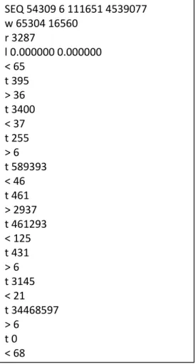
A program called pcap2tmix converts the packet capture data (pcap) file from tcpdump into tmix connection vector (tcvec) files, the primary input to Tmix. Tcvec files contain a number of tcvecs and each tcvec represents a connection from the original pcap. An example tcvec can be seen in Figure 1. The first line defines the connection as sequential (SEQ) or concurrent (CONC) depending on the timing of the packets within the connection, the start time of the connection in microseconds relative to the start time of the experiment, the number of epochs, described below, in the connection, and several identification numbers. The second line specifies the TCP window sizes, the third specifies the round trip time for the connection in microseconds, and the fourth is currently unused.

The remaining lines specify the behavior of the connection. Connections are viewed as a collection of epochs which are made up of application data units (ADUs) and think times. ADUs represent the application data objects being transferred between two parties in the original TCP connection. Think times represent the amount of time between two consecutive request-response exchanges. For example, an epoch could represent a request for a web page, the server’s response, and the time the user takes to read the page before sending another request. Lines starting with > or < indicate the amount of bytes in an ADU being sent or received by the machine that started the

connection. While processing the epochs in a tcvec, Tmix adds delay before sending each packet in order to simulate the minimum RTT specified in the tcvec’s header section.

11

By replaying tcvecs between pairs of machines, Tmix allows us to perform experiments with real-world traffic, containing any patterns or irregularities that come with it, and freeing us from the burden of determining how to create traffic patterns that match those seen on the Internet.

9. Network Setup

a. Hardware

Before we could run experiments with Tmix, we had to set up a network in our lab. A diagram of our network can be seen in Appendix A. Organized as a dumbbell, our network consists of two primary subnets: 192.168.138.x and 192.168.139.x. Both of these subnets consist of four end systems and a router plugged into a switch. The routers are connected by a link with 10.168.138.x addresses that is tapped to a machine running Endace Data Acquisition and Generation (DAG) software for capturing our network traffic during experiments. Every link in our network is 1 Gbps Ethernet with the exception of 10 Gbps fiber links between the routers. Our network is required to be isolated from the rest of UNC’s networking infrastructure, so we have an access machine, Yoda, which is connected to the Internet and both of our switches.

Each of our eight end systems run Tmix and have Intel 1 Gbps NICs, dual core Intel Pentium 4 2.80 GHz processors, and 2 GB of RAM. Both routers have Intel 1 Gbps NICs on their links to the switches and Intel 10 Gbps fiber NICs on the link between them, quad core Intel Xeon 2.00 GHz processors, and 4 GB of RAM. Our monitor machine has an Endace DAG 4.5G4 to capture traffic, two six core Intel Xeon 3.50 GHz processors, and 64 GB of RAM.

12

this, the router in our 138 subnet, Leia, had an HDD fail and we discovered the machine had been set up with a RAID configuration. As a result, we had to wipe Leia and set the machine up once again. The lesson here was to not set up machines with RAID configurations unless absolutely necessary. Had Leia not been using a RAID configuration, we would have been able to simply replace the disk and keep going. Instead, we had to reinstall the OS and start over.

We also spent a significant amount of time setting up our monitor machine. Initially, we tried to use a machine called Cypher and two Intel NICs to capture traffic using tcpdump, but discovered that Cypher did not have enough open PCI slots of the appropriate size for our NICs. After considering our options, we purchased a single Intel NIC with two sets of fiber ports. Upon receiving the NIC and installing it, the machine recognized the card, ethtool shows the link as up, but we were unable to get the card to send any packets. We had to return the card and evaluate other options. At this point in the school year, we were running low on time for setup and decided to borrow a machine named

Bloodhound, the machine whose technical specifications are listed above.

b. Software

On each of our eight end systems, we installed Ubuntu 14.04.1 LTS. The routers were configured later and have Ubuntu 14.04.2 LTS installed. We left our monitor machine in the state we borrowed it, with Ubuntu 12.04.5 LTS.

13

10. Running Experiments

To perform an experiment, Tmix is run for one hour on each of the four pairs of end systems, each pair consisting of a machine from the 138 subnet and a machine from the 139 subnet, and DAG capturing tools are run on our monitor machine. The machines in our 139 subnet replay data originating from UNC and the machines in our 138 subnet replay data originating from the rest of the Internet. All data in an experiment is sent over the fiber link between the two routers. As a result, this link emulates UNC’s ingress-egress link from which the traffic was originally captured. After running these

experiments, we use a tool developed at UNC called bpfmon that computes the average throughput in both directions across this main link.

The traffic we replay has more data originating from outside of UNC, meaning we send more data from our 138 subnet to our 139 subnet during our experiments than from 139 to 138. Because we wish to test AQMs in a congested environment, we want to run them on the most congested portion of our network. The nature of our traffic results in us running the AQMs on Leia’s fiber NIC.

11. Calibration

Our next step was to calibrate our network. We needed to make sure there were no bottlenecks during our experiments that we were not intentionally creating. Our calibration procedure operates on the idea that as the number of cvecs we replay increases, we should see an approximately linear increase in the throughput on our main link between the routers.

To test this, we generated pairs of tcvecs representing 1/30th_{, 1/15}th_{, 1/10}th_{, 1/9}th_{, 1/8}th_{, 1/7}th_,

1/6th_{, 1/5}th_{, 1/4}th_{, 1/3}rd_{, and 1/2 of the captured traffic from UNC’s ingress-egress link in addition to a}

14

systems on our network. After running these experiments, we generated the graphs in Appendix B by plotting the number of TCP connections (tcvecs) vs throughput for each experiment.

Each blue point on these graphs represents a one hour experiment replaying up to several million connections between a single pair of machines. As expected, a linear relationship between the number of tcvecs being replayed and the throughput on the main fiber link exists, as demonstrated by the black line in each graph. It is easy to see that this relationship is lost after the experiment where the machine on the 138 side of the network started 1.66 million tcvecs, the experiment representing 1/2 of the originally captured traffic from UNC’s ingress-egress link. From these graphs, we concluded that we can safely replay 1/2 of the original traffic, generating 165 Mbps in our high throughput direction, on each of our four pairs of machines. As an extra precaution, we verified that the end systems’ CPU utilization during this experiment was about 70%, an acceptable level.

12. Rate Limiting

From our calibration, we learned that each pair of machines can replay 165 Mbps in our high throughput direction, but this amounts to only 660 Mbps with all four pairs. This is not enough traffic to achieve our desired 80%, 90%, and 98% link utilization for our experiments, so we began looking into possible ways of inducing congestion by rate limiting Leia’s fiber NIC. If we could limit the rate of the NIC to speeds for which 660 Mbps represented 80%, 90%, and 98% link utilization, we could perform our experiments with just four pairs of machines.

15

them over their maximum value [4]. In our case, we wanted to use HTB to limit the rate at which any data was leaving the NIC, so we configured HTB to have a single default class to which all packets were enqueued and set that class to have our desired bandwidth.

After being directed to a page outlining current best practices for testing CoDel, we learned that experiments involving HTB should be performed with a kernel configured to run at a rate of 1000 HZ [12]. We then backported the 3.16.0-lowlatency kernel from the Ubuntu 14.10 repositories and installed it on Leia.

13. Byte Queue Limits and Network Offloads

Several other best practices included modifications to Byte Queue Limits (BQL) and network related offloads. In the Linux kernel, packets are sent from the IP Stack to the qdisc, then to the driver queue, and finally are sent by the NIC, as per the diagram in Figure 2. BQL is a feature of the Linux kernel that seeks to limit the amount of data in the driver queue to prevent queueing delay. While in

operation, BQL automatically tunes the limit of how many bytes of data should be sent to the driver queue in a given interval of time to limit the possibility of delay. BQL was created to be self-tuning at 1 Gbps and 10 Gbps link speeds, and for links under 100 Mbps, the CoDel best practices recommended setting the maximum number of bytes BQL can send to the driver queue in an interval of time to 3000, just enough for two packets. We decided we did not want to trust BQL’s auto tuning and that we should set the maximum limit to 3000 bytes as well.

16

stack to store more than a maximum transmission unit (MTU) of data in each of the data structures pointed to in the driver queue, putting the responsibility of splitting this data into MTU sized packets on the NIC. These features increase throughput by allowing significantly more data to be queued in the driver queue, but at the risk of greatly increasing queueing delay. Disabling these offloads ensures no more than an MTU worth of data can be stored in each data structure pointed to in the driver queue. This feature, combined with the limiting of the maximum number of bytes BQL can send to the driver queue in an interval of time, mitigates the risk of significant delay resulting from unexpected behavior in the driver queue. We chose to disable TSO, UFO, and GSO on Leia’s fiber NIC.

The generic receive offload (GRO) and large receive offload (LRO) are similar to their TSO, UFO, and GSO counterparts. GRO and LRO operate on incoming traffic and combine received packets before sending them to the IP stack. We chose to disable these offloads on Leia’s fiber NIC in addition to TSO, UFO, and GSO.

17

14. Preliminary Experiments with CoDel

After properly configuring HTB, setting the maximum limit for BQL, and disabling all offloads on Leia’s fiber NIC, we decided to run some preliminary experiments in preparation for my honors

presentation. Due to the limited amount of time we had before the presentation, we decided to run experiments with drop-tail and CoDel for link utilizations of 90% and 98%.

While running the experiments, we noticed our monitor machine was capturing far less traffic than expected. Upon looking at the qdisc statistics after the experiments, we noted they were reporting that approximately 42% of packets were being dropped. Looking into the cause for these unexpected drops, it appeared as though some combination of setting the maximum limit for BQL and disabling all of the offloads was to blame. We are still experimenting with these parameters and remain unsure as to the cause of the significant loss in throughput we experienced.

15. Going Forward

While we continue to investigate this loss in throughput, we have decided that the networking offloads should be disabled on every NIC in all of our machines, both routers and end systems, for our final experiments. Ideally, we want a packet to be treated as a packet and do not want to have the Linux kernel attempting to modify them for the purpose of optimization.

18

While HTB may work for rate limiting, it would be best if we could congest our link without an additional piece of software. To this end, we are adding four more pairs of machines to our network, enabling us to congest a 1 Gbps link between the routers. Unlike in our preliminary experiments, we will not adjust the rate of Leia’s fiber NIC to invoke congestion, but will alter the number of tcvecs being replayed on each machine such that all 4 pairs generate 800 Mbps, 900 Mbps, and 980 Mbps in the high throughput direction to vary the link utilization between experiments.

In addition to adding eight more end systems, we need to acquire a more recent capture of the network traffic from UNC’s ingress-egress link. Until now, calibration and experimentation have been performed with data from 2008. We will obtain data from 2015 in order to test how these AQMs will perform with modern traffic patterns.

We will also be losing access to Bloodhound, and will need to acquire a new machine for monitoring our future experiments.

19

16. Conclusions

This past year has given me a much greater appreciation for the difficulties of research and the enormous amount of patience it requires. I never would have imagined that I would spend weeks on things as seemingly trivial as replacing bad hard drives or setting up a monitor machine only to have to give up and borrow Bloodhound.

20

References

[1] Floyd, Sally. "TCP and Explicit Congestion Notification." ACM SIGCOMM Computer Communication Review 24.5 (1994): 8-23. Web.

[2] Gettys, Jim. "Bufferbloat: Dark Buffers in the Internet." IEEE Internet Computing 15.3 (2011): 96. Web.

[3] Hernandez-Campos, Felix, Kevin Jeffay, and F. Donelson Smith. "Modeling and Generating TCP Application Workloads." 2007 Fourth International Conference on Broadband

Communications, Networks and Systems (BROADNETS '07) (2007): n. pag. Web.

[4] Hubert, Bert, Gregory Maxwell, Remco Van Mook, Martijn Van Oosterhout, Paul B. Schroeder, and Jasper Spaans. "Linux Advanced Routing & Traffic Control HOWTO." Linux Advanced Routing & Traffic Control. Lartc.org, 19 May 2012. Web. 14 Apr. 2015.

[5] Khademi, Naeem, David Ros, and Michael Welzl. "The New AQM Kids on the Block: An Experimental Evaluation of CoDel and PIE." 2014 IEEE Conference on Computer Communications

Workshops (INFOCOM WKSHPS) (2014): n. pag. Web.

[6] Le, Long, Jay Aikat, Kevin Jeffay, and F. Donelson Smith. "The Effects of Active Queue Management and Explicit Congestion Notification on Web Performance." IEEE/ACM Transactions on Networking 15.6 (2007): 1217-230. Web.

[7] Nichols, Kathleen, and Van Jacobson. "Controlling Queue Delay." Queue 10.5 (2012): 20. Web. [8] Pan, R., P. Natarajan, F. Baker, B. Versteeg, M. Prabhu, C. Piglione, V. Subramanian, and G. White.

"PIE: A Lightweight Control Scheme to Address the Bufferbloat Problem." Draft-ietf-aqm-pie-01 - PIE: A Lightweight Control Scheme to Address the Bufferbloat Problem. Internet

Engineering Task Force, 26 Mar. 2015. Web. 09 Apr. 2015. Work in Progress.

21

[10] Subramanian, Vijay, and Mythili Prabhu. "PIE - Proportional Integral Controller-Enhanced AQM Algorithm." Tc-pie(8) - Linux Manual Page. Iproute2, 16 Jan. 2014. Manpage. 16 Apr. 2015. [11] Subramanian, Vijay. "CoDel - Controlled-Delay Active Queue Management Algorithm." Tc-codel(8) -

Linux Manual Page. Iproute2, 23 May 2012. Manpage. 16 Apr. 2015.

[12] Taht, Dave, and Jim Gettys. "Best Practices for Benchmarking CoDel and FQ CoDel (and Almost Any Other Network Subsystem!)." Best Practices for Benchmarking CoDel and FQ CoDel -

Bufferbloat. N.p., 1 Sept. 2014. Web. 16 Apr. 2015.

[13] Weigle, Michele C., Prashanth Adurthi, Félix Hernández-Campos, Kevin Jeffay, and F. Donelson Smith. "Tmix: A Tool for Generating Realistic Application Workloads in Ns-2." ACM SIGCOMM

Computer Communication Review 36.3 (2006): 67-76. Web.

22

Appendix A: Network Topology

A d

iag

ram

o

f t

h

e

to

p

o

lo

gy

o

f

o

u

r net

wo

rk

as

o

f Ap

ril

, 2

0

1

5

23

Appendix B: Calibration Graphs

These graphs are from calibration experiments run on a pair of machines in our network. Each blue point represents a one hour experiment replaying up to several million TCP connections. From least to greatest number of tcvecs, the experiments were performed for 1/30th_{, 1/15}th_{, 1/10}th_{, 1/9}th_{, 1/8}th_,

1/7th_{, 1/6}th_{, 1/5}th_{, 1/4}th_{, 1/3}rd_{, and 1/2 of the traffic captured from UNC’s ingress-egress link, as well as}

an experiment for the entire dataset. The black lines are drawn to show the linear relationship between all but the last of these experiments and the red lines connect each of the blue points.

A graph of the number of tcvecs vs throughput in the high

24