A Heuristic’s Job Order Gain in Pyramidal Preemptive Job Scheduling Problems for Total Weighted Completion Time Minimization

(1)

doi: 10.7250/itms-2019-0001

https://itms-journals.rtu.lv

A Heuristic’s Job Order Gain in Pyramidal

Preemptive Job Scheduling Problems

for Total Weighted Completion Time Minimization

Vadim Romanuke

Polish Naval Academy, Gdynia, Poland

Abstract – A possibility of speeding up the job scheduling by a heuristic based on the shortest processing period approach is studied in the paper. The scheduling problem is such that the job volume and job priority weight are increasing as the job release date increases. Job preemptions are allowed. Within this model, the input for the heuristic is formed by either ascending or descending job order. Therefore, an estimator of relative difference in duration of finding an approximate schedule by these job orders is designed. It is ascertained that the job order results in different time of computations when scheduling at least a few hundred jobs. The ascending-order solving becomes on average by 1 % to 2.5 % faster when job volumes increase steeply. As the steepness of job volumes decreases, this gain vanishes and, eventually, the descending-order solving becomes on average faster by up to 4 %. The gain trends of both job orders slowly increase as the number of jobs increases.

Keywords – Heuristic, job order, job parts, job scheduling, preemption, total weighted completion time minimization.

I. INTRODUCTION TO PYRAMIDAL PREEMPTIVE JOB

SCHEDULING PROBLEMS

Optimal scheduling is a very important means to efficiently executing multistage processes of manufacturing, assembling, building, rendering, dispatching, etc. Scheduling problems are addressed by the scheduling theory, which provides effective approaches to finding both exactly and approximately optimal schedules [1], [2]. An optimal schedule allows executing the process in the minimal total weighted completion time (TWCT). Job scheduling problems (JSPs), where the schedule is commonly considered without idle time intervals, are segregated in two classes, one of which allows a job to preempt, and another one does not support any preemptions [1], [3]. Preemptive JSPs (PJSPs) are also segregated in a few subclasses. One of them constitutes PJSPs, wherein the job volume and job priority weight are increasing as the job release date increases [4], [5]. These ones could be called pyramidal PJSPs (PPJSPs) whose complexity and costs grow as the process progresses [2], [3]. The PPJSP is a model of multi-sectional mounting, which is still possible by assembling “later” sections before “earlier” (i.e., simpler and cheaper) ones owing to supported preemptions.

II. RELATED WORKS AND MOTIVATION

Most JSPs are solved by using heuristics because exact schedules are found intractably slow [6], [7]. When a JSP is given by job parts (or processing periods), release dates, and priority weights, without due dates or other constraining

variables or parameters, it is effectively solved by the shortest processing period approach (SPPA) [5], [8]. This is a heuristic trying to minimize TWCT by executing the most expensive job first if it has the fewest parts to do [9]. When PJSPs are not pyramidal but all the jobs instead have the same volume [10], the heuristic finds an approximate schedule faster if the release dates are given in descending order (along with non-increasing priority weights) [5]. Namely, the descending job order input (DJOI) has a 1 % relative advantage in scheduling more than 200 jobs for such non-pyramidal PJSPs. With increasing the number of jobs off 1000, this advantage has a slight tendency to increase. Eventually, the advantage can achieve up to 22 %. Therefore, it is obvious that a maximally possible computation time gain [5], [11] is obtained in scheduling longer series of bigger-sized non-pyramidal PJSPs. The question is whether a similar gain could be obtained in solving PPJSPs.

III. THE GOAL AND TASKS

As approximately solving PPJSPs by the heuristic may be sped up, the goal is to ascertain whether the order of inputting the job release dates results in different time of computations for such JSPs. For achieving this goal, the following eight tasks are to be fulfilled:

1. To define a simplified model of PPJSPs, which will be used for computer simulations.

2. Within the defined model, to define PPJSPs by the ascending job order input (AJOI) and PPJSPs by DJOI, which must be clearly distinguished.

3. To state items of the heuristic based on the SPPA. 4. To design an estimator of relative difference in duration of solving PPJSPs by AJOI and DJOI.

5. To design a generator of random series of PPJSPs by both AJOI and DJOI.

6. To estimate the computation time of solving PPJSPs by both AJOI and DJOI using the SPPA.

7. To discuss whether the difference between the computation time of AJOI and that of DJOI is significant. The significant difference between the computation time of AJOI and that of DJOI would imply a significance of the heuristic’s job order gain (either by AJOI or DJOI).

(2)

IV. DEFINITION OF THE PPJSP

Let N be a number of jobs to be scheduled, where

 

\ 1

N . Job n is divided into H_n equal parts, where, in general, H_n . For a slight simplification, the job part is counted as a unit. Thus, job n has a processing period of H_n units, n=1,N: vector

 

₁ N

n _N

H _ P

=  

H (1)

contains all the volumes of those N jobs, where P is a special constraint imposed on the set of job parts.

Besides, job n has a release date r_n (measured similarly to the job parts) and a priority weight wn , n=1,N . Without losing generality, they are also set at integer values:

 

1

N

n N

r _ Y

=  

R , (2)

 

1

N

n N

w _ Z

=  

W , (3)

where Y and Z are special constraints imposed on the sets of job release dates and respective priority weights. Constraint Y is obligatory for job release dates inasmuch as they should be arranged into vector (2) so that no idle intervals would be produced, and at least one element in R should be equal to 1.

The class of PPJSPs is marked out by constraints P, Y ,

Z. These are the subsets, which have the following property:

1 2

n n H H and

1 2

n n w w for

1 2

n n

r r by n₁n₂, (4) wherein

  n₁ E



1,N−1



such that

1 1 1

n n

H =H ₊ by E N−1 (5)

is a partial case. Property (4), however, can hold without (5), when E= . Then such PPJSPs may be referred to as strictly PPJSPs. Another slight simplification in considering PPJSPs comes with a strict homogeneous monotonicity (SHM) in vectors (2) and (3), wherein either condition

n

r =n and w_n=n  =n 1,N (6) or

1 n

r = − +N n and w_n= − +N n 1  =n 1,N (7) holds. The direction of monotonicity (either increasing or decreasing) determines the job order input.

V. AJOI AND DJOI

Whichever subset E is, PPJSPs by AJOI are those that have condition (6). Consequently, PPJSPs by DJOI are those that have condition (7). Obviously, if this is AJOI by (6), then the volumes of those N jobs in vector (1) are non-decreasing. Inversely, the volumes in vector (1) are non-increasing for DJOI by (7). Strictly PPJSPs, for which E= , will have increasing

and decreasing job volumes for AJOI and DJOI, respectively.

VI. THE HEURISTIC BASED ON THE SPPA

The total length of the schedule measured in definite time units is

1 N

n n

T H

=



. (8)

The schedule is a set

 

1 t T s _ =

S of job numbers/tags, which are

to be executed, along the increasing T time units, where

 

1, t

s  N for every t=1,T. (9)

Set S defines N moments at which each job is completed (the last part of the job is executed). Let job n be completed after moment 

( )

n , which is 

( )

n 

 

1,T and the H_n-th part is executed at that moment. The goal is to compose such a schedule of those N jobs that it would give the minimal TWCT, which is

( )

min

1 min

N n n

n

w n

 =

 =



 . (10)

The heuristic based on the SPPA often allows finding schedules giving an exactly minimal TWCT whose value by (10) in the case of PPJSPs can be re-written as

( )

AJOI

min AJOI

1 min

N

n n

 =

 =



 =

( )

(

)

( )

DJOI

DJOI 1

min 1

N

n n

N n n

 =

=



− +  , (11)

where _AJOI

( )

n and _DJOI

( )

n are the moments at which job n is completed by a schedule after AJOI and DJOI, respectively.

Denote an approximate schedule, given by the heuristic based on the SPPA, by

 

st 1T =

S with st

 

1,N for every t=1,T. (12)

This heuristic uses a vector of the remaining processing periods (RPPs), which at the start is just equal to vector (1):

 

qn1N

= =

Q H. (13)

As time t progresses for a one time unit, one of those RPPs decreases, and thus vector (13) is changed by successive decrements. For every t=1,T a set of available jobs

( )



 

1, : _i and _i 0



 

1,

(3)

is determined, whence a set of weight-to-RPP ratios

( )

i i i A t w t

q _

 

 _{=  }

  for every t=1,T (15)

is obtained. The maximal ratio is achieved at subset

( )

_{( )}

( )

*

arg max i

i A t i w

A t A t

q



 

= _{ }

  for every t=1,T. (16)

If

( )

* 1

A t = (17)

then the decrement in vector (13) of RPPs is executed:

* t

s =i by * *

(obs)

i i

q =q and * *

(obs) 1

i i

q =q − . (18)

Otherwise, if (17) is false then

( )

* 1

A t  (19)

and a set

( )

( ) *

( )

* *

** *

arg max _i i A t

A t w A t A t



=   (20)

is found, where

( )

 

( )

 

** ** *

1 1,

L l _l

A t i A t A t N

=

=    . (21)

Then the decrement in vector (13) of RPPs is executed using the first element of set (21):

** 1 t

s =i by ** **

1 1

(obs)

i i

q =q and ** **

1 1

(obs) 1

i i

q =q − . (22)

An approximate TWCT is calculated successively for every

1,

n= N using the moments 

( )

n 

 

1,T at which job n is completed. Finally,

( )

min

1 N

n n

w n

=

 =



  (23)

is an approximately minimal TWCT that corresponds to the quasi-optimal job schedule (12).

VII. AN ESTIMATOR OF SOLVING DURATION DIFFERENCE

The duration of solving a PPJSP (i.e., its computation time) depends on the number of jobs and the set constraining the vector of job volumes. For definite N and P, let us denote averaged times of obtaining the heuristic’s schedule by AJOI and DJOI, respectively, by _AJOI

(

N P,

)

and _DJOI

(

N P,

)

. Inasmuch as the heuristic is a rapid solving, an estimation of

difference between _AJOI

(

N P,

)

and _DJOI

(

N P,

)

, ,

, 100

,

N P N P

N P

 − 

 = 

 . (24)

Obviously, a computation time gain with DJOI exists when estimator (24) is positive. If it is negative, then AJOI gives a computation time gain.

VIII. AGENERATOR OF PPJSPS BY AJOI AND DJOI

For generating random series of PPJSPs by AJOI and DJOI, constraint P should be modelled only. Thus, a stride

N s

d  

=  _ _ by d \ 1

 

and dN (25)

is taken, where function  

( )

returns the integer part of number  [4], [5], [7], and job volumes

j

H =k for k 1, N s  

=  _{ }  = +j 1 s k

(

−1 ,

)

sk (26)

by

max

j j

H =H  =j j_max+1,N when j_max s N N s   = _ _

  (27)

are generated. Then estimator (24) is refined by labelling P as

d P .

The smaller stride (25) is, the steeper the change of the job volumes becomes. For instance, the smallest stride ( s=1) given by d=N−1, produces the SHM in vector (1), wherein either condition

n

H =n  =n 1,N (28)

or

1 n

(4)

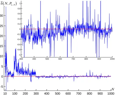
Fig. 1. Estimator (24) for the case of SHM in vector (1) by (28) and (29), where the horizontal zero level is put on. The averaging is executed over 100 PPJSPs generated for both AJOI and DJOI at every number of jobs starting from 2 through 1000. In the two additional graphs, put on as zoom-ins, computational artefacts are ignored. If to look closely, the relative advantage of AJOI seems to be slowly increasing as the number of jobs increases.

Nevertheless, the way in which job volumes increase in the (1,N)-PPJSP is too steep. Other PPJSPs generated by smaller d are also pretty “steep”. For smoothing this steepness, let an additional parameter be introduced into rule (26), which now becomes

smooth j

H = +k k by ksmooth

for k 1, N

s  

=  _{ }  = +j 1 s k

(

−1 ,

)

sk. (30)

Rule (30) will be used for generating “smoother” PPJSPs (by increasing k_smooth). They, however, will consist of “harder” jobs whose parts are increased exactly by k_smooth, which is the additional parameter along with stride (25).

IX. ANALYSIS OF THE OBTAINED RESULTS AND DECISION ON THE HEURISTIC’S JOB ORDER GAIN

The “smoothest” PPJSP is generated by d=2. Therefore, it matters to see how estimator (24) changes when the PPJSP changes from the “smoothest” to “steeper” one. Let d=2, 9

for this (Fig. 2). Here, the average estimator (AE) is (Fig. 3)

(

2...9

)

9

(

)

2 1

, ,

8_d d

N P N P

=

 =



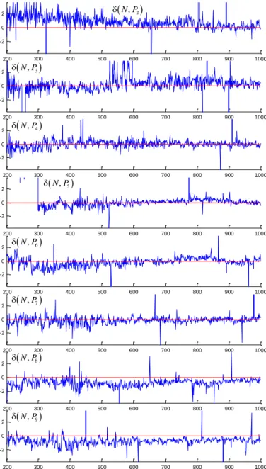
 . (31)

Although AE (31) does not really show where a job order gain could be obtained, zoom-ins on the 8 graphs of Fig. 2 shown in Fig. 4 allow making some conclusions. Indeed, DJOI has a slight advantage in solving the “smoothest” PPJSP. Then, as the steepness of job volumes increases, this advantage vanishes and, eventually, solving with AJOI becomes slightly faster (this is well seen in Fig. 4 for d=8 and d=9). For a notice, the steepness of job volumes herein is shown in Fig. 5.

Fig. 2. Estimators (24) over 100 PPJSPs, where artefacts are not cut. Artefacts are essential for a fewer hundreds of jobs due to shorter computation time.

Fig. 3. AE (31) over graphs in Fig. 2. The additional graph ignores artefacts.

10 100 200 300 400 500 600 700 800 900 1000

-5 0 5 10 15 20 25 30

300 400 500 600 700 800 900 1000

-1 -0.8 -0.6 -0.4 -0.2 0 0.2 0.4 0.6 0.8 1

(N P, 2...9)



N

10 100 200 300 400 500 600 700 800 900 1000 0

50 100

10 100 200 300 400 500 600 700 800 900 1000 -20

0 20 40

10 100 200 300 400 500 600 700 800 900 1000 -20

0 20 40

10 100 200 300 400 500 600 700 800 900 1000 0

20 40 60

10 100 200 300 400 500 600 700 800 900 1000 -20

0 20 40 60

10 100 200 300 400 500 600 700 800 900 1000 0

20 40 60 80

10 100 200 300 400 500 600 700 800 900 1000 -5



2 100 200 300 400 500 600 700 800 900 1000

0 20 40 60 80 100 120 140 160

2 100 200 300 400 500 600 700 800 900 1000 -5

0 5 10

300 400 500 600 700 800 900 1000

-2.5 -2 -1.5 -1 -0.5 0 0.5 1 1.5 2 2.5

(

N P, N−1

)



(5)

Fig. 4. The zoom-ins on the 8 graphs of Fig. 2 by cutting their artefacts off.

Fig. 5. An example of the steepness of job volumes in PPJSPs with 50 jobs by 2,9

d= (Fig. 2 and Fig. 4). Note that neither AJOI nor DJOI can be seen here.

Figure 6 confirms that “steeper” PPJSPs (by d=20, 25) are solved faster by AJOI. The AE (Fig. 7)

(

20...25

)

25

(

)

20 1

, ,

6 d

d

N P N P

=

 =



 (32)

shows that AJOI has roughly a 1 % advantage here. The zoom-ins on the 6 graphs of Fig. 6 shown in Fig. 8 confirm this conclusion but only for scheduling no less than 500 jobs.

Finally, let us generate “smoother” PPJSPs by (30) for

smooth 1, 4

k = . Let us denote estimator (24) by 

(

N P k, ₂; _smooth

)

and

(

)

(

)

smooth 4

2 2 smooth

1 1

, ; {1...4} , ;

4 k

N P N P k

=

 =



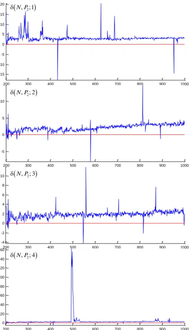
 (33)

is AE herein. Such PPJSPs are solved faster by DJOI (Fig. 9) whose gain is 2 % for scheduling 300 jobs and more (Fig. 10).

Fig. 6. Estimators (24) over 100 “steeper” PPJSPs, wherein jobs are of greater volumes than job volumes in Fig. 5, with uncut artefacts. Artefacts are lesser compared to those ones in Fig. 2 because here the computation time is longer.

50 100 200 300 400 500 600 700 800 900 1000 0

5 10

50 100 200 300 400 500 600 700 800 900 1000 -5

0 5 10

50 100 200 300 400 500 600 700 800 900 1000 -10

-5 0 5

50 100 200 300 400 500 600 700 800 900 1000 -5

0 5 10 15

50 100 200 300 400 500 600 700 800 900 1000 0

50 100

50 100 200 300 400 500 600 700 800 900 1000 -6



d

10 20 30 40 50

2 3 4 5 6 7 8 9

1 2 3 4 5 6 7 8 9 10

n n H

200 300 400 500 600 700 800 900 1000 -2

0 2

200 300 400 500 600 700 800 900 1000 -2

0 2

200 300 400 500 600 700 800 900 1000 -2

0 2

200 300 400 500 600 700 800 900 1000 -2

0 2

200 300 400 500 600 700 800 900 1000 -2

0 2

200 300 400 500 600 700 800 900 1000 -2

0 2

200 300 400 500 600 700 800 900 1000 -2

(6)

Fig. 7. AE (32) over graphs in Fig. 6. The additional graph ignores artefacts.

Fig. 8. The zoom-ins on the 6 graphs of Fig. 6 by cutting their artefacts off. Despite fluctuations, an offset below the horizontal zero level is clearly seen.

Fig. 9. The DJOI gain (with uncut artefacts) in scheduling “smoother” PPJSPs, wherein jobs of the “smoothest” PPJSPs are of 5 and 6 parts, whereas PPJSPs generated by the smallest additional parameter in (30) are of 2 and 3 parts.

Fig. 10. AE (33) over graphs in Fig. 9. The relatively huge artefact is cut in the additional graph. An increase of the AE is seen in the additional graph.

200 300 400 500 600 700 800 900 1000

0 5 10 15 20 25 30 35 40

N

(

N P, 2;{1...4}

)



200 300 400 500 600 700 800 900 1000 0

0.5 1 1.5 2 2.5 3 3.5 4 4.5 5

200 300 400 500 600 700 800 900 1000 -15

-10 -5 0 5 10 15 20

200 300 400 500 600 700 800 900 1000 -5

0 5 10

200 300 400 500 600 700 800 900 1000 -4

-2 0 2 4 6 8 10

200 300 400 500 600 700 800 900 1000 0



200 300 400 500 600 700 800 900 1000 -2

0 2

200 300 400 500 600 700 800 900 1000 -2

0 2

200 300 400 500 600 700 800 900 1000 -2

0 2

200 300 400 500 600 700 800 900 1000 -2

0 2

200 300 400 500 600 700 800 900 1000 -2

0 2

200 300 400 500 600 700 800 900 1000 -2



50 100 200 300 400 500 600 700 800 900 1000

-8 -6 -4 -2 0 2 4 6 8 10 12 14 16

(N P, 20...25)



N

100 200 300 400 500 600 700 800 900 1000 -1.5

(7)

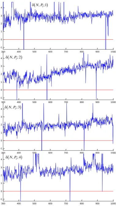
The zoom-ins on the 4 graphs of Fig. 9 shown in Fig. 11 allow asserting that this gain will continue increasing as the number of jobs increases. In scheduling more than 1000 jobs, DJOI is almost 3 % faster than AJOI (see both Fig. 10 and Fig. 11). However, the increase is not expected to be boundless. An asymptote of the increase trend in Fig. 10 does plausibly exist as well as asymptotes of the decrease trends in Fig. 1 and Fig. 7 do.

Fig. 11. The zoom-ins on the 4 graphs of Fig. 9 without their minor artefacts. The slight increase of the DJOI gain is clearly seen (the abrupt increase for

smooth 2

k = is an artefact of the increase trend itself). It is also seen that solving such PPJSPs for 1000 jobs and more is sped up by almost 3 % with DJOI.

After all, the obtained results certainly confirm that the SPPA heuristic has a definite job order gain, i.e. an approximate schedule can be found faster by using either AJOI or DJOI that depends on how steep job volumes increase in the PPJSP. Indeed, the difference between the computation time of AJOI and that of DJOI can achieve up to 3 %, whose significance is discussed below.

X. DISCUSSION

Obviously, a difference between the computation time of AJOI and that of DJOI becomes significant if scheduling along the real-time scale has a positive impact on the total system performance. If to consider just a PPJSP with even a few thousand jobs, the difference (if any) being roughly a small fraction of a second may seem negligible. Nevertheless, solving a long series of PPJSPs turns the difference into seconds, minutes, and even hours, which are ever crucial for the real-time industrial performance. Moreover, if PPJSPs are solved for organising computational processes, then speeding up by even a small fraction of a second is very important and struggled for. Therefore, notwithstanding the relatively small percentage, the SPPA heuristic’s job order gain (either by AJOI or DJOI) in solving PPJSPs is significant.

For emphasising the significance for the real practice, let a larger PPJSP be solved. The PPJSP consists of 60000 jobs, wherein every 20000 of them are divided into 4, 5, and 6 equal parts. It is a “smooth” PPJSP rather than “steep”. Using a single CPU core, without parallelizing, the computation time of DJOI here is 147 seconds, whereas solving with AJOI takes 151 seconds. Thus, DJOI has a 2.79 % relative advantage. Therefore, a series of 1000 such PPJSPs will be solved in about 400 seconds faster by DJOI. It is clear that solving longer series of such PPJSPs and similar JSPs overall saves hours!

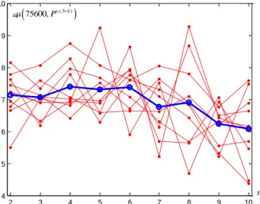
As it has been already ascertained, such an advantage decreases as the PPJSP gets “steeper”. In spite of the decrease of estimator (24), the difference between the computation time of AJOI and that of DJOI does not necessarily have a distinct decreasing feature. For instance, in solving a PPJSP consisting of 75600 jobs, wherein every 75600 s of them (s=2, 10) are divided into 3+k equal parts (k=1,s), estimator (24)

re-denoted by 

(

_75600,_P( ;3s +k)

)

_{showing the DJOI advantage} decreases (Fig. 12), but its numerator denoted by

(

( ;3 )

)

75600,Ps +k

 does not seem decreasing (Fig. 13).

Fig. 12. A set of 10 estimators and its average (the thicker line with circles) showing how the DJOI advantage decreases in solving the PPJSP as the steepness of job volumes increases. At s=2 every 37800 jobs are divided into 4 and 5 equal parts; at s=3 every 25200 jobs are divided into 4, 5, 6 equal parts; at s=10 every 7560 jobs are divided into 4, 5, 6, ..., 12, 13 equal parts.

2 3 4 5 6 7 8 9 10

1 1.5 2 2.5 3 3.5 4 4.5

s

(

_75600,_P( ;3s+k)

)



300 400 500 600 700 800 900 1000 -1

0 1 2 3 4

300 400 500 600 700 800 900 1000 -1

0 1 2 3 4

300 400 500 600 700 800 900 1000 -1

0 1 2 3 4

300 400 500 600 700 800 900 1000 -1

0 1 2 3

4 

(

N P, 2; 4

)

Fig. 13. The difference between the computation time in seconds of AJOI and that of DJOI for the set of 10 estimators in Fig. 12 (the average is a thicker line with circles). While the decreasing of the DJOI relative advantage is quite certain, the “steeper” PPJSPs herein are still solved by 6 seconds faster with DJOI.

The process of scheduling considered here is implicitly executed on a single machine [12]. Executing it on multiple machines speeds up finding an approximate schedule. In this case, the order of inputting the job release dates is naturally believed to result in different time of computations as well. However, scheduling on multiple machines does not imply straightforward parallelization like that using GPUs or CPU cores. Hence, it is not clear whether the computation time gain obtained by AJOI and DJOI for PPJSPs considered above will be repeated in the case of scheduling (by the SPPA heuristic) on multiple machines.

XI. CONCLUSION

It has been ascertained that, in solving PPJSPs by the SPPA heuristic, the order of inputting the job release dates (or priority weights) results in different time of computations when scheduling at least a few hundred jobs. If job volumes increase steeply, solving with AJOI becomes efficient. The

(1,N)-PPJSP, for example, is solved with AJOI by 1 % to 2.5 % faster. As the steepness of job volumes decreases, the AJOI gain vanishes and, eventually, solving with DJOI becomes faster by up to 4 %. The gain trends of both AJOI and DJOI slowly increase as the number of jobs increases. Nevertheless, the described heuristic’s job order gain does not necessarily happen in solving a single PPJSP, especially if the PPJSP consists of a few tens of jobs divided in a few parts each. Hence, the computation time gain by either AJOI or DJOI is obtained on average, although a computational artefact is a low-probability event. The gain significance grows for more voluminous PPJSPs. This is quite serviceable for organising computational processes, where any delays are undesirable.

ACKNOWLEDGMENT

The research has technically been supported by the Faculty of Navigation and Naval Weapons at the Polish Naval Academy, Gdynia, Poland.

REFERENCES

[1] M. L. Pinedo, Scheduling: Theory, Algorithms, and Systems. Springer International Publishing, 2016.

https://doi.org/10.1007/978-3-319-26580-3

[2] P. Brucker, Scheduling Algorithms. Springer-Verlag Berlin Heidelberg, 2007. https://doi.org/10.1007/978-3-540-69516-5

[3] M. L. Pinedo, Planning and Scheduling in Manufacturing and Services. Springer-Verlag New York, 2009.

https://doi.org/10.1007/978-1-4419-0910-7

[4] V. V. Romanuke, “The exact minimization of total weighted completion time in the preemptive scheduling problem by subsequent length-equal job importance growth,” Bulletin of V. Karazin Kharkiv National University. Mathematical Modelling. Information Technology. Automated Control Systems, iss. 40, pp. 60–66, 2018.

[5] V. V. Romanuke, “A faster way to approximately schedule equally divided jobs with preemptions on a single machine by subsequent job importance growth,” Bulletin of V. Karazin Kharkiv National University. Mathematical Modelling. Information Technology. Automated Control Systems, iss. 41, pp. 80–87, 2019.

[6] W.-Y. Ku and J. C. Beck, “Mixed Integer Programming models for job shop scheduling: A computational analysis,” Computers & Operations Research, vol. 73, pp. 165–173, 2016.

https://doi.org/10.1016/j.cor.2016.04.006

[7] V. V. Romanuke, “Accuracy of a heuristic for total weighted completion time minimization in preemptive single machine scheduling problem by no idle time intervals,” KPI Science News, no. 3, pp. 52–62, 2019.

https://doi.org/10.20535/kpi-sn.2019.3.164804

[8] H. Belouadah, M. E. Posner, and C. N. Potts, “Scheduling with release dates on a single machine to minimize total weighted completion time,”

Discrete Applied Mathematics, vol. 36, no. 3, pp. 213–231, 1992.

https://doi.org/10.1016/0166-218X(92)90255-9

[9] S. Ul Sabha, “A novel and efficient round robin algorithm with intelligent time slice and shortest remaining time first,” Materials Today: Proceedings, vol. 5, no. 5, part 2, pp. 12009–12015, 2018.

https://doi.org/10.1016/j.matpr.2018.02.175

[10] H. Wei and J. Yuan, “Two-machine flow-shop scheduling with equal processing time on the second machine for minimizing total weighted completion time,” Operations Research Letters, vol. 47, no. 1, pp. 41–46, 2019. https://doi.org/10.1016/j.orl.2018.12.002

[11] B. Wang, Y. Song, J. Cao, X. Cui, and L. Zhang, “Improving task scheduling with parallelism awareness in heterogeneous computational environments,” Future Generation Computer Systems, vol. 94, pp. 419–429, 2019. https://doi.org/10.1016/j.future.2018.11.012

[12] M. Nattaf, S. Dauzère-Pérès, C. Yugma, and C.-H. Wu, “Parallel machine scheduling with time constraints on machine qualifications,” Computers & Operations Research, vol. 107, pp. 61–76, 2019.

https://doi.org/10.1016/j.cor.2019.03.004

Vadim Romanuke graduated from the Technological University of Podillya (Ukraine) in 2001. In 2006, he received the Degree of Candidate of Technical Sciences in Mathematical Modelling and Computational Methods. The Candidate Dissertation suggested a way of increasing interference noise immunity of data transferred over radio systems. The degree of Doctor of Technical Sciences in Mathematical Modelling and Computational Methods was received in 2014. The Doctor-of-Science Dissertation solved a problem of increasing efficiency of identification of models for multistage technical control and run-in under multivariate uncertainties of their parameters and relationships. In 2016, he received the status of Full Professor.

He is a Professor of the Faculty of Navigation and Naval Weapons at the Polish Naval Academy. His current research interests concern decision making, game theory, statistical approximation, and control engineering based on statistical correspondence. He is the author of 347 scientific articles, one monograph, one tutorial, three methodical guidelines in Functional Analysis, Development of Master Theses in Mathematical and Computer Modelling, Conflict-Controlled Systems. Before January 2018, Vadim Romanuke was the scientific supervisor of a Ukrainian budget grant work concerning minimization of water heat transfer and consumption. He also leads a branch of fitting statistical approximators at the Centre of Parallel Computations in Khmelnitskiy, Ukraine. Address for correspondence: 69 Śmidowicza Str., Gdynia, Poland, 81-127. E-mail: [email protected]

ORCID iD: https://orcid.org/0000-0003-3543-3087

s

2 3 4 5 6 7 8 9 10

4 5 6 7 8 9 10

(

_75600,_P( ;3s +k)