Evaluating and Generalization of Methods of Cyclic Coordinate, Hooke Jeeves, and Rosenbrock

(1)

Evaluating and Generalization of Methods of Cyclic

Coordinate, Hooke – Jeeves, and Rosenbrock

Mohammad Ali Khandan, Mehdi Delkhosh

*

Department of Mathematics and Computer, Damghan University, Damghan, Iran *Corresponding Author: [email protected]

Abstract

In optimization problems, we are looking for best point for our problem. Problems always classify to unary or n-ary with bound or unbound. In this paper, we evaluate three methods, Cyclic Coordinate, Hooke – Jeeves, and Rosenbrock on n dimensional space for unbounded problem and we speak about the advantages and disadvantages of these three methods. We offer solutions for some disadvantages and we give generalized algorithms to improve the methods.

Keywords

Golden Section Method, Cyclic Coordinate Method, Hooke – Jeeves Method, Rosenbrock Method

1. Introduction

In optimization problems, we are looking for best point for our problem. Problems always classify to unary or n-ary with bound or unbound. There are several methods for optimization problems, such that Cyclic Coordinate method, Hooke - Jeeves method, and Rosenbrock method on n dimensional space for unbounded problem.

Here, we consider the problem of minimizing a function f

of several variables without using derivatives. The methods described here proceed in following manner. Given a vector x, a suitable direction d is first determined, and then f is minimized from x in the direction d by one of the techniques we will describe.

Direct search methods are suitable tools for maximizing or minimizing functions that are non-smooth and non-differentiable. In their comprehensive book about non-linear programming [7] mention three methods (multidimensional search methods without using differentiating): the cyclic coordinate method, the Hooke-Jeeves method, and the Rosenbrock method. The cyclic coordinate method alters the value of one decision variable at a time, i.e. coordinate axes as the search directions. The Hooke-Jeeves method uses two search modes: exploratory search in the direction of coordinate axes (one decision variable altered at a time) and pattern search in other directions (more than one decision variable altered

simultaneously). The method of Rosenbrock tests m (m is the number of optimized decision variables) orthogonal search directions which are equal to coordinate axes only at the first iteration. Rosenbrock search is a numerical optimization algorithm applicable to optimization problems in which the objective function is inexpensive to compute and the derivative either does not exist or cannot be computed efficiently.

Another type of method, namely dynamic programming, has been used extensively in stand management optimization [8]. It differs from direct search methods so that, instead of seeking optimal values for continuous decision variables, it finds the optimal sequence of stand states defined by classified values of several growing stock characteristics (for instance, basal area, mean diameter, and stand age).

Direct search methods can be used in both even-aged and uneven-aged forestry [9]. Uneven-aged management can also be optimized using linear programming and a transition matrix model [10]. Of the direct search methods mentioned in [7] the Hooke-Jeeves algorithm has been used much in forestry, at least in Finland [11, 12].

In this paper, we first introduce these three methods, and then we express the advantages and disadvantages them, and finally, we give generalized algorithms to improve them.

2. The Method of Cyclic Coordinate

In this method we move on Coordinate axes as much as

λ

until get the optimal point [1, 4, and 6].

2.1. Algorithm for Cyclic Coordinate Method Initial step:

Choose a scalar

ε

>

0

to be used for terminating the algorithm. And let

d

1

,

d

2

,...,

d

n _{be the Coordinate} directions. Choose an initial point

x

₁ , let

y

₁

=

x

₁, let

1 =

=

j

k

and got to the main step. Main Step:

(2)

minimize

  

ℜ ∈

+

λ

) (

f yj dj Min

, and let

j j j

j

y

d

y

₊₁

=

+

λ

. if

j

<

n

, replace j by j+1, and repeat step 1. Otherwise if

j

=

n

go to step 2. 2. Let

x

k+₁

=

y

k+₁. If

x

k+1

−

x

k

<

ε

then stop.

Otherwise let

y

1

=

x

k+1

,

j

=

1

, replace k by k+1 and

repeat step 1.

2.2. Advantages of Cyclic Coordinate Method 1. Implementation of an algorithm is simple.

2. We can use this algorithm for functions that either is differentiable or are not differentiable.

2.3. Disadvantages of Cyclic Coordinate Method

1. When we use this method for differentiable functions, it will converge to a point with zero gradients. But when the function is not differentiable, the method may stall at a non-optimal point.

2. This method converts an n-ary function to a unary, and by using an algorithm for solving unary function gain an optimal point and set in the n-ary function. Then increase the overhead of the algorithm.

3. We solve a unary system in each step and should pay attention to the domain of unary system. If the domain does not have a minimum point then the system does not get a good solution.

2.4. Checking problems of Cyclic Coordinate Method 2.4.1. Problem 1

Hooke - Jeeves algorithm is proposed to solve the first problem

2.4.2. Problem 2

The simplex method is used to solve the second problem (It must be considered that the complexity of the simplex method is not better than this)

2.4.3. Problem 3

Consider the following problem that solve according to the Cyclic Coordinate method.

We use the Golden section method (see Appendix) for solving unary system. The method initial with a uncertainty interval and we know minimum point is in this range. At each step decrease the range until gets a good range. Now imagine we have several extremum points or don’t have any minimum point in this range. Then we check this special state in following sample.

2 2 1

2 2 1 4 1 2 1

)

,

(

.

)

2 (

)

2 (

)

,

(

ℜ

∈

−

+

−

=

x

t

s

x

f

Min

Start point:

)

3 ,

0 (

1

₌

x

,

0 .

2

1

0 ,

0

1

2

1

₌













=













=

d

ε

d

In first step unary function shows like this with the following values (Figure 1):

)

3 ,

0 (

1

₌

y













=

0

1

d

4 2

1

)

(

6 )

(

2 )

(

y

+

λ

d

=

−

+

λ

+

−

+

λ

[image:2.595.314.554.166.420.2]

f

Figure 1. let _y1₌₍₀_,₃_),_d1₌₍₁_,₀₎t

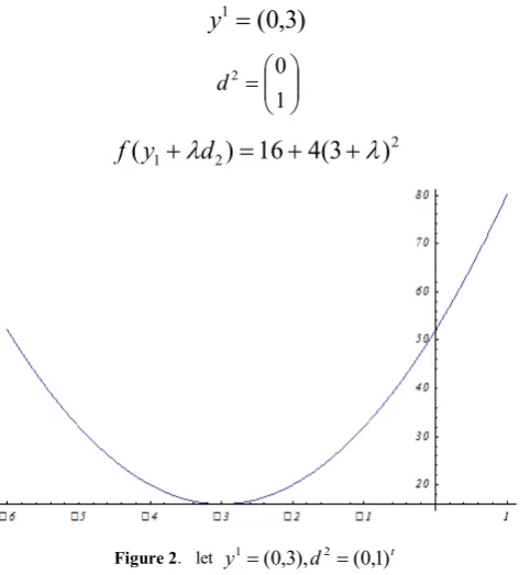
In second step unary function shows like this with the following values (Figure 2):

)

3 ,

0 (

1

₌

y

      =

1 0 2

d

2 2

1

)

16

4 (

3 )

(

y

+

λ

d

=

+

λ

[image:2.595.315.552.458.720.2]

f

Figure 2. let _y1₌₍₀_,₃_),_d2₌₍₀_,₁₎t

(3)

becomes large or small.

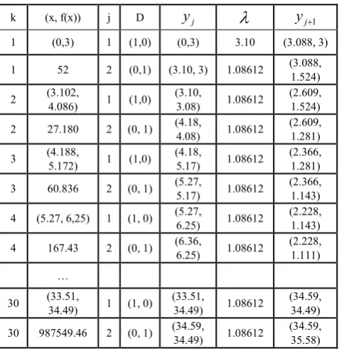
[image:3.595.60.296.132.326.2]

Now if run the algorithm with an initial range (-4, 4) for Golden section method [2], we get following data in table 1.

Table 1. Run the algorithm of Cyclic Coordinate with initial (-4, 4)

K (x, f(x)) j d

y

_j

λ

y

j+₁

1 (0,3) 1 (1, ₀₎ (0,3) 3.088 (3.088, 3)

1 52 2 (0, ₁₎ (3.088, 3) -1.475 (3.088, _1.524)

2 (3.088, _1.524) 1 (1, ₀₎ (3.088, _1.524) -0.478 (2.609, _1.524)

2 1.403 2 (0, ₁₎ (2.609, _1.524) -0.242 (2.609, _1.281)

3 (2.609, _1.281) 1 (1, ₀₎ (2.609, _1.281) -0.242 (2.366, _1.281)

3 0.140 2 (0, ₁₎ (2.366, _1.281) -0.137 (2.366, _1.143)

4 (2.366, _1.143) 1 (1, ₀₎ (2.366, _1.143) -0.137 (2.228, _1.143)

4 0.024 2 (0, ₁₎ (2.228, _1.143) -0.032 (2.228, _1.111)

We could find answers in iteration 4.

But if we choice initial range (1, 6) for Golden section method then have following data in table 2.

As you can see table 2, not only doesn’t close to minimum point but reach to a larger number at each step and get away from the optimal point. So in thirtieth iteration x is (33.51, 34.49) and there are many differences between this number and the number of the previous table. The algorithm doesn’t halt at this point and we can continue for iteration 31 and so on.

If you look at the table 2, at each iteration we use the Golden section method,

λ

is 1.08612. In fact almost consider beginning of the range.

Table 2. Run the algorithm of Cyclic Coordinate with initial (1, 6)

k (x, f(x)) j D

y

_j

λ

y

j+₁

1 (0,3) 1 (1,0) (0,3) 3.10 (3.088, 3)

1 52 2 (0,1) (3.10, 3) 1.08612 (3.088, _1.524)

2 (3.102, _4.086) 1 (1,0) (3.10, _3.08) 1.08612 (2.609, _1.524)

2 27.180 2 (0, 1) (4.18, _4.08) 1.08612 (2.609, _1.281)

3 (4.188, _5.172) 1 (1,0) (4.18, _5.17) 1.08612 (2.366, _1.281)

3 60.836 2 (0, 1) (5.27, _5.17) 1.08612 (2.366, _1.143)

4 (5.27, 6,25) 1 (1, 0) (5.27, _6.25) 1.08612 (2.228, _1.143)

4 167.43 2 (0, 1) (6.36, _6.25) 1.08612 (2.228, _1.111)

…

30 (33.51, _34.49) 1 (1, 0) (33.51, _34.49) 1.08612 (34.59, _34.49)

30 987549.46 2 (0, 1) (34.59, _34.49) 1.08612 (34.59, _35.58)

2.5. Modifications to Algorithm of Cyclic Coordinate Method (Solution for Problem 3)

For solving this problem, we should find critical points for the Golden section algorithm. We need to differentiate from function in order to find critical point, and examine the state of function in previous and next points of where the function has a zero gradient. So we can’t implement this job for following reasons:

1. We're working on that function may not be differentiable.

2. In each step we should apply another algorithm in order to specify a critical area in the Golden section method. So this job increase running time of main algorithm and it may not be cost effective.

3. Differentiating from function is complex.

4. If we can differentiate from function, and find the minimum point when has a zero gradient, then we don’t need trouble yourself and implement the algorithm because we have minimum point!!!!!

3. The Method of Hooke - Jeeves

In this method we move on Coordinate axes until get optimal point [5, 6, and 7].

3.1. Algorithm for Hooke - Jeeves Method Initial step:

Choose a scalar

ε

>

0

to be used in terminating the algorithm, and

d

1

,

d

2

,...,

d

n _{as Coordinate directions.} Choose a starting point

x

₁, let

y

₁

=

x

₁ . Let

k

=

j

=

1

and go to the main step.

Main step:

1. Let

λ

j be an optimal solution to the problem to

minimize

  

ℜ ∈

+

λ

) (

f yj dj Min

, and let

j j j

j

y

d

y

₊₁

=

+

λ

. if

j

<

n

j

=

n

, let

x

k+₁

=

y

k+₁.

If

x

k+1

−

x

k

<

ε

then stop, otherwise go to step 2.

2. Let

d

=

x

_k+1

−

x

_kand find optimal solution of

problem and consider this solution is

_λ

ˆ

. Let

1 ,

ˆ

1

=

x

+

d

j

=

y

k

λ

, replace

k

by

k

+

1

and

repeat step 1.

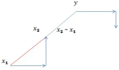
[image:3.595.59.298.507.755.2]

(4)

[image:4.595.81.275.124.239.2]

coordination, we have a search on direction of

x

₂

−

x

₁. So this job speeds up reaching to optimal solution. Look at figure 3.

Figure 3. Search on direction of x2−x1for speed up

3.2. Advantages

We haven’t placed in the trap of hole by introducing acceleration step.

3.3. Disadvantages

1. As you see, we also search in the direction of

x

₂

−

x

₁ in order to speed up the algorithm in step 2. But we don’t examine halting condition when move in this direction. Maybe the algorithm has the necessary condition for halting when move in this direction, while we run algorithms for the next iteration. This job increase running time of the algorithm.

2. We always search in the direction of the Coordinate

directions in Cyclic Coordinate and Hooke - Jeeves algorithms. Now do speed up algorithms if we do searching on other vectors?

3. In this method, we convert an n-ary function to an unary function and by algorithms for unary system find optimal point and set this optimal point an n-ary system. So this job increases running time of algorithm.

4. We should note that to the domain of unary system when we want to solve this system. If minimum is not in this domain, we don’t have a proper solution.

3.4. Checking Problems of Hooke - Jeeves Algorithm We examine Hooke - Jeeves algorithm for following example.

2 2 1

2 2 1 4 1 2 1

)

,

(

.

)

2 (

)

2 (

)

,

(

ℜ

∈

−

+

−

=

x

t

s

x

f

Min

Start point:

)

3 ,

0 (

1

₌

x

2 .

0 ,

1

0 ,

0

1

2

1

₌













=













=

d

ε

d

[image:4.595.65.548.478.633.2]

From Golden section method used for solving unary system. Initial uncertainty interval for the inner Golden section method [2] is (-4, 4).

Table 3. Run the algorithm of Hooke - Jeeves with initial (-4, 4)

d yj

λˆ +

λ

ˆ

d

1

+ j

y

j

λ

j

d

j

y

j

(x, f(x)) k

- -

- (3.08, 3)

3.08 (1, 0)

(0, 3) 1

(2.66, 1.72) -.13

(3.08, -1.47) (3.08, 1.52)

-1.47 (0, 1)

(3.08, 3) 2

52 1

- -

- (2.69, 1.72)

0.03 (1, 0)

(2.66, 1.72) 1

(3.08, 1.52) 2

(2.13, 1.01) 1.40

(-0.39, -0.20) (2.69, 1.31)

-0.41 (0, 1)

(2.69, 1.72) 2

1.40 2

- -

- (2.00, 1.01)

-0.13 (1, 0)

(2.13, 1.01) 1

(2.69, 1.31) 3

(1.90, 0.94) 0.13

(-0.69, -0.32) (2.00, 0.98)

-0.03 (0, 1)

(2.00, 1.01) 2

(5)

As you see in table 3, algorithm stop in three steps by halting condition 0.2 what we can say it works better that Cyclic Coordinate.

Now we want to modify algorithm a little. Means instead examine halting condition in step 1, examine that in step 2.

Generalized algorithm is like this:

3.5. Generalized Algorithm for Hooke – Jeeves Method (Algorithm 2)

Initial step:

Choose a scalar

ε

>

0

to be used in terminating the algorithm, and

d

1

,

d

2

,...,

d

n _{as Coordinate directions.} Choose a starting point

x

₁, let

y

₁

=

x

₁ . Let

k

=

j

=

1

and go to the main step.

Main step:

1. Let

λ

minimize   

ℜ ∈

+ λ

λ )

( f yj dj Min

. And let

j j j

j

y

d

y

₊₁

=

+

λ

. if

j

<

n

j

=

n

, let

x

k+₁

=

y

k+₁

and go to step 2.

2. Let

d

=

x

_k+1

−

x

_k and find the optimal solution of

the problem and consider this solution is

_λ

ˆ

. Let

d

x

y

1

=

k+1

+

λ

ˆ

and go to step 3.

3. Let

x

k

=

x

k+₁and

x

k+1

=

y

1. If

x

k+1

−

x

k

<

ε

stop. Otherwise let j=1 , replace k by k+1 and repeat step 1.

Now run this algorithm for previous example.

[image:5.595.66.548.326.469.2]

As you can see in table 4, the numbers are equals with past examples. But anyway running time of this algorithm is lower that first algorithm.

Table 4. Run the Generalized algorithm (2) of Hooke - Jeeves with initial (-4, 4)

d yj

λˆ +

λ

ˆ

d

1

+ j

y

j

λ

j

d

j

y

j

(x, f(x)) k

- -

- (3.08, 3)

3.08 (1, 0)

(0, 3) 1

(2.66, 1.72) -0.13

(3.08, -1.47) (3.08, 1.52)

-1.47 (0, 1)

(3.08, 3) 2

52 1

- -

- (2.69, 1.72)

0.03 (1, 0)

(2.66, 1.72) 1

(3.08, 1.52) 2

(2.13, 1.01) 1.40

(-0.39, -0.20) (2.69, 1.31

-0.41 (0, 1)

(2.69, 1.72) 2

1.40 2

- -

- (2.00, 1.01)

-0.13 (1, 0)

(2.13, 1.01) 1

(2.69, 1.31) 3

(1.90, 0.94) 0.13

(-0.69, -0.32) (2.00, 0.98)

-0.03 (0, 1)

(2.00, 1.01) 2

0.23 3

3.6. Generalized Algorithm for Hooke – Jeeves Method (Algorithm 3)

In previous algorithms, we move along Coordinate directions in order to reach an optimal point. Now do we reach to an optimal solution if we move along other linear independent vectors?

According to considered example on space

_ℜ

2_{we want to move in the direction of orthogonal and linear independent}

[image:5.595.65.547.575.721.2]

vectors (1,2) and (-2,1) in order to reach an optimal point. Now we run the algorithm in the direction of these two vectors:

Table 5. Run the Generalized algorithm (3) of Hooke - Jeeves with initial (-4, 4)

d yj

λˆ +

λ

ˆ

d

1

+ j

y

j

λ

j

d

j

y

j

(x, f(x)) k

- -

- (-0.08, 2.83)

-0.08 (1, 2)

(0, 3) 1

(2.67, 1.46) -0.0001

(2.67, -1.53) (2.67, 1.46)

-1.37 (-2, 1)

(-0.08, 2.83) 2

52 1

- -

- (2.54, 1.19)

-0.13 (1, 2)

(2.67, 1.46) 1

(2.67, 1.46) 2

(1.82, 0.93) 1.88

(-0.29, -0.18) (2.37, 1.27)

0.08 (-2, 1)

(2.54, 1.19) 2

0.26 2

- -

- (1.82, 0.93)

0.0002 (1, 2)

(1.82, 0.93) 1

(2.37, 1.27) 3

(1.82, 0.93) -0.0001

(-0.55, -0.34) (1.82, 0.93)

-0.0001 (-2, 1)

(1.82, 0.93) 2

0.05 3

(6)

4. The Method of Rosenbrock

In this method we search to in direction of n linearly independent and orthogonal vectors in each iteration. When we reach to a new point on each iteration, we construct a new set of orthogonal vectors [3, 6].

4.1. Algorithm for Rosenbrock Method Initial step:

Let ε>0 be the termination scalar. Choose _d1_,_d2_,...,_dn

as coordinate directions. Choose a starting point

x

₁ , let

1 1

x

y

=

, k= j=1 and go to the main step. Main step:

1. Let

λ

minimize   

ℜ ∈

+

λ

λ )

( f yj dj Min

setyj+1=yj+

λ

jdj. If

n

j

<

, replace j by j+1 and repeat step 1. Otherwise, go to step 2.

2. Let

x

k+1

=

y

k+1 . If

x

k+1

−

x

k

<

ε

then stop.

Otherwise, let

y

₁

=

x

k+₁ and replace k by k+1 , let

j=1 and go to step 3.

3. From a new set of linearly independent orthogonal search directions by term 1. Denote these new directions by

d

1

,

d

2

,...,

d

n and repeat step 1.

4.2. Term 1

Let

d

1

,

d

2

,...,

d

n be linearly independent vectors. Each

with a norm equal to 1. Furthermore, suppose that these vectors are mutually orthogonal, that is

d

ti

.

d

j

=

0

for

i

≠

j

.

Starting from the current vector

x

k, the objective function

f

is minimized along each of the directions iteratively,

resulting in the point

x

k+₁ . In particular,

∑

=

+

−

=

n

j j j

k

x

d

x

1

λ

Where

λ

j_{is the distance moved along}

d

j_{. The new}

collection of directions

d

1

,

d

2

,...,

d

n _{is formed by the}

Gram-Schmidt procedure or orthogonalization procedure, as follow:

   

≠ =

=

_∑

= 0

0

j n

j

i i i

j j

j _d _if

if a

a

_λ

λ

   

≥ −

= =

∑

−

=

2 ) )( . (

1 1

1

j if d d a a

j if a

b j

i i i

t j j

j

j j

j

_b

b

d

=

4.3. Running Rosenbrock Algorithm

We examine Rosenbrock algorithm for following example

2 2 1

2 2 1 4 1 2 1

)

,

(

.

)

2 (

)

2 (

)

,

(

ℜ

∈

−

+

−

=

x

t

s

x

f

Min

Start point:

)

3 ,

0 (

1

₌

x

, 0.2

1 0 , 0 1 ₂

1 ₌

      =      

= d

ε

d

We use a Golden section method for solving unary system. Initial interval of uncertainty for inner golden section method [2] is (-4,4).

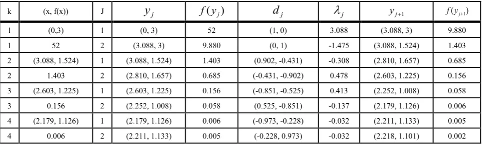
[image:6.595.64.548.579.725.2]

Data for this example are in table 6.

Table 6. Run the algorithm of Rosenbrock with initial (-4, 4)

k (x, f(x)) J

y

_j

f

(

y

_j

)

d

_j

λ

_j yj+1 f(yj+1)

1 (0,3) 1 (0, 3) 52 (1, 0) 3.088 (3.088, 3) 9.880

1 52 2 (3.088, 3) 9.880 (0, 1) -1.475 (3.088, 1.524) 1.403

2 (3.088, 1.524) 1 (3.088, 1.524) 1.403 (0.902, -0.431) -0.308 (2.810, 1.657) 0.685 2 1.403 2 (2.810, 1.657) 0.685 (-0.431, -0.902) 0.478 (2.603, 1.225) 0.156 3 (2.603, 1.225) 1 (2.603, 1.225) 0.156 (-0.851, -0.525) 0.413 (2.252, 1.008) 0.058 3 0.156 2 (2.252, 1.008) 0.058 (0.525, -0.851) -0.137 (2.179, 1.126) 0.006 4 (2.179, 1.126) 1 (2.179, 1.126) 0.006 (-0.973, -0.228) -0.032 (2.211, 1.133) 0.005 4 0.006 2 (2.211, 1.133) 0.005 (-0.228, 0.973) -0.032 (2.218, 1.101) 0.002

(7)

5. Numerical Example for Each Three

Methods and Comparing Them

In this section, we examine other problem for three methods, Cyclic Coordinate, Hooke - Jeeves and Rosenbrock. And contrast these three methods.

Problem: 2 2 1 2 2 1 2 2 1 2 1

)

,

(

.

)

(

5 )

1 (

)

,

(

ℜ

∈

−

+

−

=

x

t

s

x

f

Min

Start point: ) 0 , 2 ( 1₌

x , 0.2

1 0 , 0 1 2 1 ₌       =      

= d ε

d

We will use golden section method for solving unary system.

Initial interval of uncertainty for inner golden section method is (-0.5, 0.5).

[image:7.595.311.552.250.483.2]

Diagram of the problem is in figure 4:

Figure 4. Diagram of 2 2 1 2 2 1 2

1, ) (1 ) 5( )

(x x x x x

f = − + −

We can’t move to an optimal solution, when we want to solve this problem by Rosenbrock method. And in each stage we take away from an answer.

For most of problems we have same complexity and same solution for each of these three methods, Cyclic Coordinate, Hooke - Jeeves and Rosenbrock. You should note that we use unary method for solving unary system in these algorithms, like Golden section method. But we need to an interval of uncertainty in unary problem, so minimum point is in this range. Most of time finding interval of uncertainty are hard, because we should know critical area of problem. So this case is impossible in non-differentiable problems.

[image:7.595.66.547.531.731.2]

Data by Cyclic Coordinate method are in table 7:

Table 7. Data by Cyclic Coordinate method

K (x, f(x)) j d

y

_j

λ

y

j+₁

1 (2, 0) 1 (1, 0) (2, 0) -0.42 (1.57, 0)

1 81 2 (0, 1) (1.57, 0) -0.10 (1.57, -0.10)

2 (1.57, -0.1) 1 (1, 0) (1.57, -0.10) -0.42 (1.14, -0.10)

2 33.48 2 (0, 1) (1.14, -0.10) -0.10 (1.14, -0.20)

3 (1.14, -0.20) 1 (1, 0) (1.14, -0.20) -0.42 (0.71, -0.20)

3 11.49 2 (0, 1) (0.71, -0.20) -0.10 (0.71, -0.30)

4 (0.71, -0.30) 1 (1, 0) (0.71, -0.30) -0.42 (0.29, -0.30)

4 3.43 2 (0, 1) (0.29, -0.30) -0.10 (0.29, -0.40)

5 (0.29, -0.40) 1 (0.29, -0.40) -0.42 (0.19, -0.40)

5 1.69 2 (0.19, -0.40) 0.10 (0.19, -0.50)

Data by Hooke - Jeeves method are in table 8:

Table 8. Data by Hooke - Jeeves method

(8)

6. Conclusions

There are many algorithms for solving optimization problems, that they have the advantages and disadvantages. We can use the generalized algorithms and corrections of algorithms in this paper, to improve other algorithms. And we get a more accurate answer. And we can use these generalized methods for more complex functions.

Appendix

1. Golden Section Method

The following is a summary of the Golden section method for minimizing a strictly quasiconvex function over the interval [a1,b1]

Initial Step:

Choose an allowable final length of uncertainty

l

>

0

. Let [a1,b1] be the initial interval of uncertainty. And let

) )( 1

( 1 1

1

1=a + −α b −a

λ and

µ

1=a1+

α

(b1−a1) , where

618 . 0 =

α . Evaluate θ(λ1) and θ(µ1). Let k=1, and go to

the main step.

Main Step:

1. If bk −ak <l, stop; the optimal solution lies in the

interval [ak,bk]. Otherwise, if

θ

(

λ

k

)

>

θ

(

µ

k

)

go to

step 2; and if

θ

(

λ

k

)

≤

θ

(

µ

k

)

go to step 3.

2. Let ak+1=λkand

b

k+1

=

b

k. Furthermore, let k

k µ

λ₊₁= _{, and let}µk+1=ak+1+α(bk+1−ak+1). Evaluate θ(µk+1) and go to step 4.

3. Let ak+1=akand

b

k+1

=

µ

k. Furthermore, let k

k λ

µ+1= , and let λk+1=ak+1+(1−α)(bk+1−ak+1).

Evaluate θ(λk+1) and go to step 4.

4. Replace k by k+1 and go to step 1.

2. Programs for the Four Methods

We implement Golden section, Cyclic Coordinate, Hooke - Jeeves, Rosenbrock methods by C# programming language.

These programs are presented as follow:

2.1. Program of Golden Section Method: public class GoldenSection

{

public int index;

private const double alfa = 0.618; public double L;

public double a; public double b;

public double landa; public double miuo; public double f_landa; public double f_miuo; public double answer; public double f_answer; //variables that used in function public double[] y = new double[2]; public double[] d = new double[2];

//... public GoldenSection(double l)

{

index = 0; //alfa = 0.618; L = l;

a = 0; b = 0; landa = 0; miuo = 0; f_landa = 0; f_miuo = 0; }

//... public void initialStep()

{

landa = a + (1.0 - alfa) * (b - a); miuo = a + (alfa * (b - a)); f_landa = function1(landa); f_miuo = function1(miuo); index = 1;

}

//... public void mainStep()

{

//int yy = 7; if ((b - a) < L) {

answer = (a + b) / 2;

f_answer = function1(answer); return;

}

else if (f_landa > f_miuo) {

step2(); }

else if (f_landa <= f_miuo) {

step3(); } }

//... public void step2()

{

(9)

miuo = miuo = a + (alfa * (b - a)); f_miuo = function1(miuo); step4();

}

{ //a = a; b = miuo; miuo = landa; f_miuo = f_landa;

landa = a + ((1.0 - alfa) * (b - a)); f_landa = function1(landa); step4();

}

{ index++; mainStep(); }

//... public double function1(double x)

{

double result = 0;

//double temp1 = (x * d[0]) + y[0] - 2;

//double temp2 = ((d[0] - 2 * d[1]) * x) + y[0] - (2 * y[1]); double temp1 = y[0] + (x * d[0]) - 2;

double temp2 = y[0] + (x * d[0]) - (2 * (y[1] + x * d[1])); result = Math.Pow(temp1, 4) + Math.Pow(temp2, 2); return result;

} }

2.2. Program of Cyclic Coordinate Method public class Cyclic Coordinate

{

public const double epsilon = 0.2; public double[] d1 = { 1, 0 }; public double[] d2 = { 0, 1 }; public double[] x;

public double[] y; public double f_x; public int j; public int k; public double landa; public DataTable dataTable;

//... public Cyclic Coordinate(double[] input) {

x = new double[2]; y = new double[2];

x = (double[])input.Clone(); f_x = 0;

j = 0; k = 0;

landa = 0;

dataTable = new DataTable(); dataTable.Columns.Add("k"); dataTable.Columns.Add("x f(x)"); dataTable.Columns.Add("j"); dataTable.Columns.Add("d"); dataTable.Columns.Add("y(j)"); dataTable.Columns.Add("landa"); dataTable.Columns.Add("y(j+1)"); }

{

y = (double[])x.Clone(); k = 1;

j = 1; }

//... public bool mainStep()

{

double[] tempY = new double[2]; while (j <= 2)

{

GoldenSection gs = new GoldenSection(0.2); gs.a = 1;

gs.b = 6;

gs.y = (double[])y.Clone(); if (j.Equals(1))

{

gs.d = (double[])d1.Clone(); }

else {

gs.d = (double[])d2.Clone(); }

gs.initialStep();

//while ((gs.b - gs.a) > gs.L) // {

gs.mainStep(); // }

int yy = 9; //answer

landa = gs.answer; if (j.Equals(1)) {

tempY = (double[])y.Clone(); y[0] = tempY[0] + (landa * d1[0]); y[1] = tempY[1] + (landa * d1[1]);

dataTable.Rows.Add(k, "(" + x[0] + " , " + x[1] + ")", j,"("+d1[0]+" , "+d1[1]+")", "(" + tempY[0] + " , "

+ tempY[1] + ")", landa, "(" + y[0] + " , " + y[1] + ")"); }

else if (j.Equals(2)) {

(10)

f_x = function(x);

dataTable.Rows.Add(k, f_x, j, "(" + d2[0] + " , " + d2[1] + ")", "(" + tempY[0] + " , " + tempY[1] + ")",

landa, "(" + y[0] + " , " + y[1] + ")"); }

j++; }

return step2(); }

//... public bool step2()

{

double[] tempX = new double[2]; tempX = (double[])x.Clone(); x = (double[])y.Clone(); //Norm 2

double[] minusX = new double[2]; minusX[0] = x[0] - tempX[0]; minusX[1] = x[1] - tempX[1]; double norm2 = Norm2(minusX); if (norm2 < epsilon)

{

return false; }

else {

y = (double[])x.Clone(); j = 1;

k++; return true; }

}

//... public double Norm2(double[] param) {

double temp = Math.Pow(param[0], 2) + Math.Pow(param[1], 2);

double result = Math.Sqrt(temp); return result;

}

//... public double function(double[] x) {

double result = 0;

double temp1 = (x[0] - 2); double temp2 = x[0] - (2 * x[1]);

result = Math.Pow(temp1, 4) + Math.Pow(temp2, 2); return result;

} }

2.3. Program of Hooke – Jeeves Method public class HookeAndJeeves

{

public const double epsilon = 0.2; public double L = 0.2;

public double[] dj1 = { 1, 0 }; public double[] dj2 = { 0, 1 }; public double[] x;

public double[] x_previous; public double[] y;

public double f_x; public int j; public int k; public double landa; public DataTable dataTable; public int indexDataTable; double[] d = new double[2]; double answer = 0;

double[] tempY = new double[2]; double a = -4;

double b = 4;

//... public HookeAndJeeves(double[] input)

{

x = new double[2];

x_previous = new double[2]; y = new double[2];

x = (double[])input.Clone(); x_previous = (double[])x.Clone(); f_x = 0;

j = 0; k = 0; landa = 0;

dataTable = new DataTable(); dataTable.Columns.Add("k"); dataTable.Columns.Add("x f(x)"); dataTable.Columns.Add("j"); dataTable.Columns.Add("y(j)"); dataTable.Columns.Add("d(j)"); dataTable.Columns.Add("landa"); dataTable.Columns.Add("y(j+1)"); dataTable.Columns.Add("d");

dataTable.Columns.Add("landa_had");

dataTable.Columns.Add("y(j) + landa_had*d"); indexDataTable = -1;

}

{

j = 1; }

{

//double[] tempY = new double[2]; while (j <= 2)

{

GoldenSection gs =new oldenSection(L); gs.a = a;

(11)

{

gs.d = (double[])dj1.Clone(); }

else {

gs.d = (double[])dj2.Clone(); }

gs.initialStep(); gs.mainStep(); landa = gs.answer; if (j.Equals(1)) {

tempY = (double[])y.Clone(); y[0] = tempY[0] + (landa * dj1[0]); y[1] = tempY[1] + (landa * dj1[1]); indexDataTable++;

dataTable.Rows.Add(k, "(" + x[0] + " , " + x[1] + ")", j, "("+ tempY[0]+" , "+tempY[1] + ")",

"(" + dj1[0] + " , " + dj1[1] + ")", landa, "(" + y[0] + " , " + y[1] + ")", "_", "_", "_");

//j++; }

else if (j.Equals(2)) {

tempY = (double[])y.Clone(); y[0] = tempY[0] + (landa * dj2[0]); y[1] = tempY[1] + (landa * dj2[1]); f_x = function(x);

} j++; } j = 2;

//different from Cyclic Coordinate //double[] tempX = new double[2]; x_previous = (double[])x.Clone(); x = (double[])y.Clone();

if (!haltCondition(x_previous, x)) {

return false; }

else { step2(); return true; }

}

//... public bool haltCondition(double[] a, double[] b) {

double[] minus = new double[2]; minus[0] = b[0] - a[0];

minus[1] = b[1] - a[1];

double norm2 = Norm2(minus); if (norm2 < epsilon)

return false;

else return true; }

//... public double Norm2(double[] param)

{

double temp = Math.Pow(param[0], 2) + Math.Pow(param[1], 2);

}

{

//double[] d = new double[2]; d[0] = x[0] - x_previous[0]; d[1] = x[1] - x_previous[1];

GoldenSection gs2 = new GoldenSection(L); gs2.a = a;

gs2.b = b; gs2.d = d;

gs2.y = (double[])x.Clone(); gs2.initialStep();

gs2.mainStep();

//double answer = gs.landa; answer = gs2.answer; //answer == landa_had double[] y2 = new double[2]; y2[0] = x[0] + (answer * d[0]); y2[1] = x[1] + (answer * d[1]); indexDataTable++;

dataTable.Rows.Add(k, f_x, j, "(" + tempY[0] + " , " + tempY[1] + ")", "(" + dj2[0] + " , " + dj2[1] + ")", landa, "(" + y[0] + " , " + y[1] + ")", "(" + d[0] + " , " + d[1] + ")", answer, "(" + y2[0] + " , " + y2[1] + ")");

y = (double[])y2.Clone(); k++;

j = 1; }

//... public double function(double[] x)

{

double result = 0;

} }

2.4. Program of Rosenbrock Method public class Rosenblock

{

public const double epsilon = 0.2; public double L = 0.2;

(12)

public double[] dj2 = { 0, 1 }; public double[] x;

public double[] y;

public double[] temp_y = new double[2]; public double[] x_previous;

public double f_x; public double f_y; public double f_temp_y; public int j;

public int k;

public double landa1; public double landa2; public DataTable dataTable; double a = -4;

double b = 4;

//... public Rosenblock(double[] input)

{

x = new double[2]; y = new double[2];

x = (double[])input.Clone(); //x_previous = (double[])x.Clone(); dataTable = new DataTable(); dataTable.Columns.Add("k"); dataTable.Columns.Add("x f(x)"); dataTable.Columns.Add("j"); dataTable.Columns.Add("y(j)"); dataTable.Columns.Add("f(y(j))"); dataTable.Columns.Add("d(j)"); dataTable.Columns.Add("landa(j)"); dataTable.Columns.Add("y(j+1)"); dataTable.Columns.Add("f(y(j+1))"); }

{

j = 1; }

{

while (j <= 2) {

GoldenSection gs = new GoldenSection(L); gs.a = a;

gs.b = b;

{

gs.d = (double[])dj1.Clone(); gs.initialStep();

gs.mainStep(); landa1 = gs.answer;

temp_y = (double[])y.Clone(); y[0] = temp_y[0] + (landa1 * dj1[0]);

y[1] = temp_y[1] + (landa1 * dj1[1]); f_temp_y = function(temp_y); f_y = function(y);

dataTable.Rows.Add(k, "(" + x[0] + " , " + x[1] + ")", j, "(" + temp_y[0] + " , " + temp_y[1] + ")", f_temp_y, "(" + dj1[0] + " , " + dj1[1] + ")", landa1 , "(" + y[0] + " , " + y[1] + ")", f_y); }

else if(j.Equals(2)) {

gs.d = (double[])dj2.Clone(); gs.initialStep();

gs.mainStep(); landa2 = gs.answer;

temp_y = (double[])y.Clone(); y[0] = temp_y[0] + (landa2 * dj2[0]); y[1] = temp_y[1] + (landa2 * dj2[1]); f_temp_y = function(temp_y); f_y = function(y);

f_x = function(x);

dataTable.Rows.Add(k, f_x, j, "(" + temp_y[0] + " , " + temp_y[1] + ")", f_temp_y, "(" + dj2[0] + " , " + dj2[1] + ")", landa2 , "(" + y[0] + " , " + y[1] + ")", f_y);

} j++; } //Step 2

x_previous = (double[])x.Clone(); x = (double[])y.Clone();

bool result = haltCondition(x_previous, x); if (!result)

return false; else {

y = (double[])x.Clone(); k++;

j = 1; step3(); return true; }

}

//... public bool haltCondition(double[] a, double[] b) {

double[] minus = new double[2]; minus[0] = b[0] - a[0];

minus[1] = b[1] - a[1];

double norm2 = Norm2(minus); if (norm2 < epsilon)

return false; else return true; }

//... public double Norm2(double[] param)

{

(13)

}

{

double[] aj1 = new double[2]; double[] aj2 = new double[2]; double[] bj1 = new double[2]; double[] bj2 = new double[2]; //1

//set a

if (landa1.Equals(0)) {

aj1 = (double[])dj1.Clone(); }

else {

aj1[0] = (landa1 * dj1[0]) + (landa2 * dj2[0]); aj1[1] = (landa1 * dj1[1]) + (landa2 * dj2[1]); }

//set b

bj1 = (double[])aj1.Clone(); double bj1Norm2 = Norm2(bj1); dj1[0] = (double)(bj1[0] / bj1Norm2); dj1[1] = (double)(bj1[1] / bj1Norm2); //2

//set a

if (landa2.Equals(0)) {

aj2 = (double[])dj2.Clone(); }

else {

aj2[0] = landa2 * dj2[0]; aj2[1] = landa2 * dj2[1]; }

//set b

bj2[0] = aj2[0] - (((aj2[0] * dj1[0]) + (aj2[1] * dj1[1])) * dj1[0]);

bj2[1] = aj2[1] - (((aj2[0] * dj1[0]) + (aj2[1] * dj1[1])) * dj1[1]);

double bj2Norm2 = Norm2(bj2); dj2[0] = (double)(bj2[0] / bj2Norm2); dj2[1] = (double)(bj2[1] / bj2Norm2); //mainStep();

}

//... public double function(double[] x)

{

double result = 0;

} }

REFERENCES

[1] J. Kiefer, Sequential minimax search for a maximum, Proceedings of the American Mathematical Society 4 (3): 502–506, 1953.

[2] W.H. Press, S.A. Teukolsky, W.T. Vetterling, and B.P. Flannery, Section 10.2. Golden Section Search in One Dimension, Numerical Recipes: The Art of Scientific Computing (3rd ed.), New York: Cambridge University Press, ISBN: 9780521880688, 2007.

[3] H.H. Rosenbrock, An Automatic Method for Finding the Greatest or the Least Value of a Function, Comput. J., Vol. 3, 1960.

[4] Kholostova, Internal resonance in an autonomous Hamiltonian system close to a system with a cyclic coordinate, Journal of Applied Mathematics and Mechanics, Vol. 66, Issue 3, pp. 357–370, 2002.

[5] R. Hooke, and T.A. Jeeves, Direct Search Solution of Numerical and Statistical Problems, J Association computer Machinery, Vol. 8, pp. 212-226, 1961.

[6] J.E. Dennis, R.B. Schnabel, Numerical Methods for Unconstrained Optimization and Nonlinear Equations (Classics in Applied Mathematics), Society for Industrial and Applied Mathematics, ISBN: 9780898713640, 1987 [7] M.S. Bazaraa, H.D. Sherali, and C. M. Shetty, Nonlinear

Programming: Theory and Algorithms, John Wiley & Sons, ISBN: 9781118626306, 2013.

[8] H.M. Hoganson, J.G. Borges, and Y. Wei, Coordinating management decisions of neighboring stands with dynamic programming, In: von Gadow, K. & Pukkala, T. (eds.). Designing green landscapes. Managing Forest Ecosystems, Vol. 15, pp. 187–221, 2008.

[9] A. Trasobares, T. Pukkala, Optimising the management of uneven-aged Pinus sylvestris L. and Pinus nigra Arn. mixed stands in Catalonia, north-east Spain, Annals of Forest Science, Vol. 61, pp. 747–758, 2005.

[10] I. Kaya, J. Buongiorno, Economic harvesting of uneven-aged northern hardwood stands under risk, Forest Science, Vol. 33, pp. 889–907, 1987.

[11] J. Miina, T. Pukkala, Using numerical optimization for specifying individual-tree competition models, Forest Science, Vol. 46(2), pp. 277–283, 2000.