http://dx.doi.org/10.4236/wjet.2015.32006
A Lumped-Parameter Model for Nonlinear
Waves in Graphene
Hamad Hazim
1, Dongming Wei
2, Mohamed Elgindi
1, Yeran Soukiassian
11Texas A & M University at Qatar, Doha, Qatar 2Nazarbayev University, Astana, Kazakhstan
Email: [email protected], [email protected]
Received 1 February 2015; accepted 14 April 2015; published 17 April 2015
Copyright © 2015 by authors and Scientific Research Publishing Inc.
This work is licensed under the Creative Commons Attribution International License (CC BY). http://creativecommons.org/licenses/by/4.0/
Abstract
A lumped-parameter nonlinear spring-mass model which takes into account the third-order elas-tic stiffness constant is considered for modeling the free and forced axial vibrations of a graphene sheet with one fixed end and one free end with a mass attached. It is demonstrated through this simple model that, in free vibration, within certain initial energy level and depending upon its length and the nonlinear elastic constants, that there exist bounded periodic solutions which are non-sinusoidal, and that for each fixed energy level, there is a bifurcation point depending upon material constants, beyond which the periodic solutions disappear. The amplitude, frequency, and the corresponding wave solutions for both free and forced harmonic vibrations are calculated analytically and numerically. Energy sweep is also performed for resonance applications.
Keywords
Graphene, Resonance, Nonlinear Vibration, Phase Diagram, Frequency Sweep
1. Introduction
E D
σ = + (1)
where is the axial strain,
σ
the axial stress, E the Young’s modulus,2 max 4 E D
σ
= − the third-order
elastic stiffness constant, and σmax the ultimate yield stress of the graphene. It appears that recent studies in literature have not incorporated the constant D into their models for the vibration analysis of graphene layers. The main objective of this work is to model and understand how graphene behaves in free and forced axial vibrations and to calculate the nonlinear resonance frequencies based on Equation (1). To initiate this study, a simplified nonlinear spring model is derived based on the lumped parameter method. We show that the third- order elastic stiffness D plays an important role in modeling the patterns of graphene in axial vibration. Within a range of the initial energy, we show that there exist periodic solutions similar to the ones obtained using the corresponding linear models and that the free oscillations are nearly sinusoidal. However, as the initial energy approaches a threshold level, the limiting free oscillations deviate drastically from the sinusoidal oscil- lations predicted by linear models. Our initial results provide some quantitative regimes in which a grap-hene resonator can operate near harmonic and non-harmonic motions. The initial results of this project provide some insight information and data on the patterns of axial vibration of a graphene monolayer which can be useful for design of graphene-based resonators. By extending this simple nonlinear spring-mass model to more realistic models, it is possible to provide new design guide to help make more efficient resonators and wave guides, shorten the design cycle and provide more accurate assessment of the mechanical behavior of these devices. In Section 2, we derive the nonlinear spring lumped parameter model from the nonlinear wave equation of a graphnene sheet under axial vibration; in Section 3, we study the existence of periodic solutions by using phase plane analysis and perturbation techniques; in Section 4, we compute the approximate analytical solutions of free vibrations using the two-scales splitting method and obtain the associated natural frequencies and ampli- tudes and compare to numerical results; in Section 5, we compute numerical solutions of forced vibrations and obtain frequency sweeps.
2. The Nonlinear Lumped Parameter Model
A graphene sheet with uniform cross-section in axial vibration with fixed-free ends can be modeled by sub- stituting (1) into the standard balance of momentum equation ρu=σ ′+f to obtain the following nonlinear wave equation subject to initial and boundary conditions :
(
)
( )
( )
( )
( )
( )
( )
0( )
, , 0, , 0
, 0 , , 0 0, 0,
0, 0, , 0
u Eu D u u f x t x L t
u x u u x x L
u t u L t
ρ
= ′′+ ′ ′′+ ∈ >
= = ∈ = ′ =
(2)
Here, we use u for second order time derivative of u and u′ for spatial derivative of u. The core- sponding steady state problem with a concentrated load of magnitude f0 at the tip x=L is
(
)
(
)
( )
( )
( )
0 0, 0,
0 0, 0
Eu D u u f x L x L
u u L
δ ′′+ ′ ′′+ − = ∈ ′ = =
(3)
where δ
(
x−L)
is the Dirac delta function. Assuming that f0 ≤σmax, the exact solution of (3) can be found by integrating (3) and applying the boundary conditions. First, we integrate from 0 to x<L and then from x to L and using σ( )
0,t =σ( )
x t, , for x<L we get:( )
max 0 0 max max 0 0 max 21 1 , 0
2
1 1 , 0
f x f E u x f x f E σ σ σ σ
− + >
= − + − ≤ (4)
( )
u L as:(
)
( )
0 ,
u L
f EX D X X X
L
= − + = (5)
Our lumped parameter model is based on assuming that the density function is given by
( )
x m(
x L)
ρ = δ − (6)
For fixed time t, integrating the equation Eu D u u
(
)
[
f0 mu]
δ
(
x L)
0′
′′+ ′ ′ + − − = over
[
0,L]
gives:( )
( )
( )
( )
( )
0 max 0 max 0 max 0 max , 21 1 , , 0
,
, 2
1 1 , , 0
f mu L t
L f mu L t
E u L t
f mu L t
L f mu L t
E σ σ σ σ −
− + − >
= − − + − − ≤ (7)
Equation (7) gives the following nonlinear spring-mass equation
( )
( )
0
, , u L t
mX EX D X X f t X
L
= + + =
(8)
The corresponding autonomeous equation of (8) in which u L t
( )
, is denoted by x, is given by: 0D
mx Ex x x
L
+ + =
(9)
m is the lumped-mass at the tip of the sheet, E is the first order stiffness and D is the thrid-order stiffness constant in (1). Using the change of variable t E
mτ
= we obtain the equivalent non-dimensional equation
0
x+ −x x x =
(10)
where max 4 E Lσ =
is a positive parameter.
3. Existence of Periodic Solutions of Free Vibration
We will show that for given initial conditions x
( )
0 and x( )
0 , Equation (10) has periodic solutions for certain range of . To determine the ranges of for which existence of periodic solutions occur, we examine the phase diagrams associated with the Equation (10) defined by:2 2
2 1
2 2 3
y x
x x C
−
= + + (11)
where y=x.
We make the following observations:
1) The y-intercepts associated with (11) are y= ± 2C , 2) C represents the energy at initial position x=0, 3) when =0, the phase diagrams are the circles 2 2
2
y +x = C with center
(
0, 0)
and radius 2C . We prove that for any C>0, there exists 0 such that for ≤ 0 Equation (10) has a periodic solution and for > 0 there exists no periodic solutions of (10). Since periodic solutions of (10) correspond to closed curves of the phase diagram, we need to examine the x-intercepts of (11) and their dependence on the equation parameters. The x-intercepts of (11) are the zeros of:( )
2 1 22 3
x
which is an even function. Therefore it is enough to consider f x
( )
, for x>0. Some properties of f x( )
are:( )
0 0f =C> ; f′
( )
x >0 for x>1 and f′
( )
x <0 for1 x<
, since
f
′
( )
x
=
x x
(
−
1
)
; and2
1 1
6 f = − C
. Based on these properties we can distinguish the following three cases (corresponding to
Figures 1(a)-(c)):
Case (a): 1 1 0
6C f
> ⇒ > ⇒
No periodic solution.
Case (b): 1 1 0
6C f
= ⇒ = ⇒
Only one x-intercept and there is a periodic solution.
Case (c): 1 1 0
6C f
< ⇒ < ⇒
Two x-intercepts and there is a periodic solution.
We conclude that the bifurcation point for a given C>0, is 0 1 6C
=
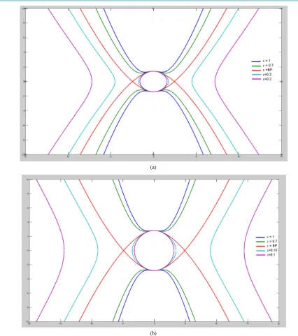
, see Figure 2.
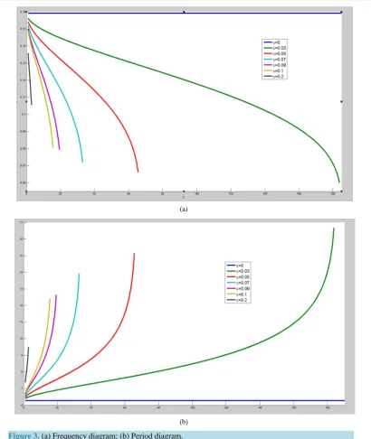
Furthermore, for each when periodic solution exists, we determine the frequency and the period numerically (see Figure 3).
It is demonstrated in Figure 2 that at a lower energy level
(
C=1)
the free vibration is approximately sinu- soidal, however at a higher level of energy(
C=4)
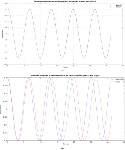
the free vibration deviate drastically from the sinusoidal pattern which has not been captured by previous models that do not include the third order elastic constant D. When periodic solutions exist, Figure 3 indicates that our model shows that at each fixed energy level, the frequency and period of a given graphene sheet depend nonlinearly on the parameter which depend on the material elastic constants as well as the length of the sheet.4. Double Scales Analytical Approximations of Free Vibration
Multiple scales method is often used to solve nonlinear equations with small parameters in nonlinear vibrations. Double scales are used herein to find an approximate solution of the first order for Equation (10). The solution is then compared to results obtained by numerical integration using Matlab. The new time scales are T0 =t,
Figure 1.
2 2
1 1
2 3
x
y=− + x x + for (a) =1, (b) 1 6 =
[image:4.595.112.519.456.718.2](a)
(b)
Figure 2. (a) Phase diagrams for C=1 and different values of ; (b) Phase diagrams for C=4 and different values of
.
1
T =t where T0 represents the fast time and T1 represents the slow time. The derivative with respect to t will be written as function of the derivative with respect to T0, T1:
0 1
2 2 2 2
2
2 2 2
0 1
0 1
,
2 .
t T T
T T
t T T
∂ = ∂ + ∂
∂ ∂ ∂
∂ = ∂ + ∂ + ∂
∂ ∂
∂ ∂ ∂
(12)
[image:5.595.93.520.77.559.2](a)
(b)
Figure 3. (a) Frequency diagram; (b) Period diagram.
sought to have the following form
(
)
(
)
( )
0 0, 1 1 0, 1
x=x T T +x T T +O (13) Substituting (13) in (10) and identifying the term of the same power of we obtain the following system of initial value problems:
( )
( )
2 0
0 0 0 0
2 0
0, 0 , 0 0 x
x x a x
T
∂ + = = =
∂ (14)
( )
( )
2 2
0 1
1 0 0 1 1
2
0 1 0
2 x , 0 0, 0 0 x
x x x x x
T T T
∂
∂ + = − + = =
∂ ∂
∂ (15)
[image:6.595.109.520.78.565.2]( )
(
( )
)
(
)
(
( )
)
(
)
( )
(
(
)
(
( )
)
)
(
)
( )
(
(
)
(
( )
)
)
0 1 0 1
0 0
1 1 0 1 0 1
0 0 0 1 2 2 2 0 0 0 1 2 2 2 cos , 2
cos cos 3 3
6π
4 1 1
cos 2 1
π 1 2 1 4 1
4 1 1
cos 2 1 ,
π 1 2 1 4 1
k
k
k
k
x a T T T
a a
x T T T
a a
k T T
k k
a a
k T T
k k
ϕ
α γ ϕ
ϕ ϕ +∞ = +∞ = = + = + + + − − + + − − + − − − + − − −
∑
∑
(16)where a T
( )
1 =a0 and( )
1 4 0 1 3πa
T T
ϕ =− . The solution of Equation (10) will then be given by:
( )
(
)
(
)
( )
(
)
(
)
( )
(
)
0 0 0 0
0 1 1
0 0 0
2 2
2
0 0 0
2 2
2
4 2 4
cos 1 cos cos3 1
3π 6π 3π
4 1 1 4
cos 2 1 1
π 1 2 1 4 1 3π
4 1 1 4
cos 2 1 1
π 1 2 1 4 1 3π
k
k
k
k
a a a a
x t a t t t
a a a
k t
k k
a a a
k t k k α γ +∞ = +∞ = = − + + + − − − + − − − + − − − − − − −
∑
∑
, (17)• The solution of Equation (14) has the following form:
( )
(
( )
)
0 1 cos 0 1
x =a T T +
ϕ
T (18) Substituting x0 in (15) and writing x0 as the Fourier series:(
0)
( )
2(
(
0)
)
1
1 2 4
cos cos 2
π π 4 1
k
k
T k T
k
ϕ +∞ ϕ
=
−
+ = − +
−
∑
the following equation is obtained
( )
(
)
( )
(
( )
)
(
( )
)
( )
(
(
( )
)
)
(
( )
)
2 1 11 0 1 0 1 0 1
2
1 1
0
0 1 0 1
2 1
2
2 sin 2 cos cos
π
4 1
cos 2 cos .
π 4 1
k
k
a T
x a
x T T a T T T T
T T
T
a
k T T T T
k
ϕ
ϕ ϕ ϕ
ϕ ϕ ∞ = ∂ ∂ + = ∂ + + + + + ∂ ∂ ∂ − − + + −
∑
(19)To avoid unbounded solutions, we set the secular terms of the x1-Equation (19), containing cos
(
T0+ϕ( )
T1)
and sin(
T0+ϕ( )
T1)
to zero. This gives the system:( )
( )
( )
0 1 1 1 0, 0 42 0, 0 0
3π a a a T a a T a T ϕ ϕ ∂ = = ∂ ∂ + = = ∂
whose solution gives a T
( )
1 =a0 and( )
1 4 0 1 3π a aT T
ϕ = − . The solution for x0 is then obtained by returning to the original time using T1=t.
To find x1, we need to solve the linear differential equation:
( )
(
(
( )
)
)
(
( )
)
(
( )
)
( )
( )
2
0 0 0 0
1
1 0 1 0 1 0 1
2 2
2 0
1 1
4 1 2
cos 2 cos cos 3 ,
π 4 1 3π
0 0, 0 0.
k
k
a a a a
x
x k T T T T T T
T k
x x
ϕ ϕ ϕ
and obtain (16), where α1 and γ1 are determined easily from the initial conditions. Using t instead of T0 and t instead of T1 and replacing a and ϕ by its values, the expression in Equation (17) is verified.
Remark
The solution for x1 shows an odd multiple of the
(
T
0+
ϕ
( )
T
1)
, this can be seen clearly in the expression for 1x . These frequencies are the harmonics of the main mode or frequency. It is a typicall feature of nonlinear differential equations that the harmonics are related directly to the nonlinear terms. Our expressions are verified numerically by calculating the solution in the frequency domain using the fourier transform and comparing with the analytical results. The results in time and frequency domains are shown below in Figure 4 and Figure 5.
(a)
(b)
[image:8.595.111.517.194.681.2](a)
(b)
Figure 5. (a) FFT of the nonlinear solution compared to the linear solution for =0.6 and x
( )
0 =0.6. (b) Linear solution compared to nonlinear numerical solution for =0.6 and x( )
0 =0.6.5. Nonlinear Vibration under Harmonic Excitation
In this section we characterize the nonlinear spring Equation (10) by a harmonic excitation and studying the system’s nonliear responses. The equation of motion is given by:
( )
( )
( )
2 cos , 0 0, 0 0
x+ +x ξ x− x x = f ωt x = x =
(20)
[image:9.595.116.515.83.589.2]near the resonnance of the coresponding linear frequency of the equation x+ =x 0. We present the numerical solutions in time and frequency domains and demonstrate the use of the frequency sweep method in detecting the nonlinear resonnance of the system.We solve Equation (20) using Matlab solver to obtain numerical results in the time domain. FFT algorithm is then applied to the time signal to find the frequencies of the solutions. The expected frequency corresponds to the excitation
ω
, the nonlinear resonance and some harmonics. The double scales method can be used to find analytical approximate solution of Equation (20) similar to the autonomeous system case of Section 4. We present our numerical results in Figure 6.We use the frequency sweep method to detect nonlinear resonnance of the nonlinear system by direct intergration. The method begins by defining a grid of frequencies around the linear resonnace and intergrate the
(a)
(b)
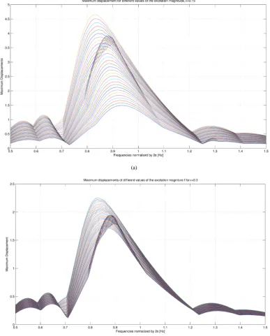
[image:10.595.122.509.204.701.2]system at each point of frequency. The maximum displacement of the solution is then plotted against the fre- quency mesh. The curve shows a peak corresponding to the nonlinear resonnance of the system. The numerical results show the dependence of the nonlinear frequency on the magnitude of excitation and on the parameter . Figure 7 and Figure 8 show the numerical results for some values of the system parameters.
6. Conclusion
A simplistic nonlinear spring model is derived from the axial wave equation of a graphene sheet based on the
(a)
[image:11.595.120.508.193.675.2](b)
(a)
(b)
Figure 8. (a) Frequency sweep for different values of at the same magnitude f . (b) Frequency sweep for the linear system for different values of f .
quadratic constitutive stress-strain equation. Using phase plane analysis, existence of periodic wave solutions and bifurcation points depending on the parameter
max 4
E Lσ
=
are verified for free vibrations. Perturbation method of time scales depending on is used to study axial vibrations subject to harmonic excitation. The results are compared with the corresponding linear spring model which does not include the third order elastic constant
2
max 4
E D
σ
[image:12.595.120.516.84.578.2]parameter critically affects the solutions quantitatively and numerically, therefore we conclude that the third order elastic constant D in the continuum mechanics based modeling of graphene should be included in further study of the dynamic behavior if higher accuracy of solutions are desired. In future studies we plan to examine the axial vibrations corresponding to the full model (2) numerically using finite differences, finite element and numerical bifurcation techniques. In addition, we plan to examine the vertical vibrations using nonlinear beam and plate equations.
Acknowledgements
The paper’s first co-author acknowledges the funding provided by the NPRP grant 08-777-1-141 from the Qatar National Research Fund (a member of Qatar Foundation) to Prof. Prabir Daripa of Texas A& M University at College Station, TX 77842, USA while working on this project.
References
[1] Dai, M.D., Kim, C.-W. and Eom, K. (2012) Nonlinear Vibration Vehavior of Graphene Resonators and Their Applica-tions in Sensitive Mass Detection. Nanoscale Research Letters, 7, 499-509.
http://dx.doi.org/10.1186/1556-276X-7-499
[2] Suggs, M.E. (2012) Graphene Resonators—Analysis and Film Transfer. Sandia Report, SAND2012-4433, Unlimited Release. http://prod.sandia.gov/techlib/access-control.cgi/2012/124433.pdf
[3] Lee, C., Wei, X.D., Kysar, J.W. and Hone, J. (2008) Measurement of the Elastic Properties and Intrinsic Strength of Monolayer Graphene. Science, 321, 385-388. http://dx.doi.org/10.1126/science.1157996
[4] Cadelano, E. (2010) Graphene under Strain. A Combined Continuum—Atomistic Approach. Ph.D. Thesis, Universita’ Degli Studi Di Cagliari, Cagliari. http://veprints.unica.it/532/1/PhD_Emiliano_Cadelano.pdf
[5] Cadelano, E., Palla, P.L., Giordano, S. and Colombo, L. (2009) Nonlinear Elasticity of Monolayer Graphene. Physical Review Letters, 102, 1-4. http://dx.doi.org/10.1103/PhysRevLett.102.235502