Modelling of the Turkish Catastrophe Insurance Pool data, 2000 2003

University of London

Modelling of the Turkish Catastrophe

Insurance Pool Data, 2000-2003

Berna Burcak Basbug

London School of Economics and Political Science

lbmitted in fulfillment of the requirements for obtaining the degree of Doctor of Philosophy

°partm ent of S tatistics, Houghton Street, London W C2A 2A E

February 2007

Library

British Library o f P o litica l

and E c o n o m ic S c i e n c e 1

UMI Number: U226803

All rights reserved

INFORMATION TO ALL USERS

The quality of this reproduction is dependent upon the quality of the copy submitted.

In the unlikely event that the author did not send a complete manuscript and there are missing pages, these will be noted. Also, if material had to be removed,

a note will indicate the deletion.

Dissertation Publishing

UMI U226803

Published by ProQuest LLC 2014. Copyright in the Dissertation held by the Author. Microform Edition © ProQuest LLC.

All rights reserved. This work is protected against unauthorized copying under Title 17, United States Code.

ProQuest LLC

Acknowledgem ents

I am grateful to my supervisor Professor Henry P. Wynn for his encouragement, wisdom, knowledge, patience, kindness and support during all my studies.

My love and special thanks to my dearest mother, Mrs.Oya Manav Ba§bug, for her love, support and patience.

I would like to thank to Professor Ozta§ Ayhan for his support, help and kindness during my Ph.D process.

I would like to thank to Assc. Prof. A. Sevtap Kestel for introducing me to the field of earthquakes, always supporting me in my career and being like a real sister to me.

Esther Heyhoe, Imelda Noble, Ulla Jakobsen, Lyn Grove and Thomas Hewitt at the London School of Economics, Department of Statistics made my life much easier during my PhD. I would like to thank to everybody at the Department of Statistics at the University of Warwick. Special thanks goes to Mrs. Paula Matthews for being a good friend and a great administrator. Thanks to Middle East Technical University Statistics department secretary Mrs. Ne§e Bilal for all her administrative help during my leave abroad.

My dearest friends, Ms. Simla Igmez and Ms. Ozlem Bay were always with me at the days full of stress, happiness and sadness for past five years. I love you both.

My very special thanks goes to Ms. Judith Anzures-Cabrera for always being there for me, for her great friendship and help with the submission of the thesis. Muchos muchos besos! Thanks to Ms. Chrysoula Dimitrou-Fakalou for being a very great friend full of wisdom and trust. Special thanks to Mr. Neil Course, Mr. Costas Kallis, Mr. Mahmut Kutlukaya, Mr. Ibrahim Erkan and Ms. Burgin Akgiin for their valuable help during my studies. I would like to thank Sultan, Ieda, Shanshan, Bruno and Milena for all their support and hospitality. Thanks to Mr. Imran Ayoob and Mr. M. Gokhan Erdamar for their help during the printing and submission process.

Acknowledgements

I am grateful to my supervisor Professor Henry P. Wynn for his encouragement, wisdom, knowledge, patience, kindness and support during all my studies.

My love and special thanks to my dearest mother, Mrs.Oya Manav Ba§bug, for her love, support and patience.

I would like to thank to Professor Ozta§ Ayhan for his support, help and kindness during my Ph.D process.

I would like to thank to Assc. Prof. A. Sevtap Kestel for introducing me to the field of earthquakes, always supporting me in my career and being like a real sister to me.

Esther Heyhoe, Imelda Noble, Ulla Jakobsen, Lyn Grove and Thomas Hewitt at the London School of Economics, Department of Statistics made my life much easier during my PhD. I would like to thank to everybody at the Department of Statistics at the University of Warwick. Special thanks goes to Mrs. Paula Matthews for being a good friend and a great administrator. Thanks to Middle East Technical University Statistics department secretary Mrs. Ne§e Bilal for all her administrative help during my leave abroad.

My dearest friends, Ms. Simla Igmez and Ms. Ozlem Bay were always with me at the days full of stress, happiness and sadness for past five years. I love you both.

My very special thanks goes to Ms. Judith Anzures-Cabrera for always being there for me, for her great friendship and help with the submission of the thesis. Muchos muchos besos! Thanks to Ms. Chrysoula Dimitrou-Fakalou for being a very great friend full of wisdom and trust. Special thanks to Mr. Neil Course, Mr. Costas Kallis, Mr. Mahmut Kutlukaya, Mr. Ibrahim Erkan and Ms. Burgin Akgiin for their valuable help during my studies. I would like to thank Sultan, Ieda, Shanshan, Bruno and Milena for all their support and hospitality. Thanks to Mr. Imran Ayoob and Mr. M. Gokhan Erdamar for their help during the printing and submission process.

F

Library

B asic research is what I am doing when I donft know what

I am doing. —Werhner von Braun

Certum ex incertis (C erta in ty out o f uncertainty). —The

British Institute of Actuaries

A bstract

C ontents

1 Introduction 20

2 Earthquakes 23

2.1 Historical view ... 23

2.2 Introduction to Turkish E a rth q u a k e s ... 31

2.2.1 Hazard Profile of T u rk e y ... 31

2.2.2 The History of Earthquakes in Turkey ...33

2.3 17/August/1999 Marmara (Kocaeli) E arth q u ak e...35

3 D istribution Theory 41 3.1 Poisson P ro c e ss...41

3.1.1 Homogeneous and Inhomogeneous Poisson Process... 41

3.2 The total claim amount (aggregate claims) process ... 47

3.2.1 The Risk Reserve and Premiums ... 51

3.2.2 Insurance/Reinsurance... 55

3.3 The Distribution of the Aggregate Claims ...58

3.3.1 Moment Generating Function (m g f)... 58

3.4 Extreme Value T h e o r y ...67

3.4.1 Moment Generating Function of the Extreme Value Distribu­ tions ... 71

3.4.2 Explanatory EVT Data Analysis of the Turkish Catastrophe Insurance Pool data between 2000-2003 ... 73

4.1.1 Likelihood of time ... 82

4.2 The use of shock k e r n e ls ... 84

4.2.1 The use of the exponential kernel in the time likelihood . . . . 91

4.2.2 The use of the power kernel in the time likelihood... 93

4.3 Generalised Linear M o d els... 94

4.3.1 Non-linear m odels... 96

4.3.2 Estimation of the non-linear parameter (3...97

4.4 Estimation of the model parameters for Poisson likelihood ...100

4.4.1 (3 derivatives...100

4.4.2 a derivatives ... 105

4.4.3 a (3 d e riv a tiv e s... 108

4.5 Estimation of the model parameters for Normal likelihood ...I l l 4.5.1 (3 derivatives... I l l 4.5.2 a derivatives ... 113

4.5.3 a (3 d e riv a tiv e s... 115

5 The D ata and M odelling 119 5.1 Turkish Earthquake Insurance Claims Data ... 119

5.2 Explanatory Analysis of the TCIP D a t a ... 122

5.3 Modelling over tim e ... 131

5.3.1 Sim ulation... 158

6 M odelling w ith Covariates 163 6.1 Graphical analysis ... 163

6.2 M o d ellin g ... 173

7 Disaster Risk M anagement 195 7.1 Natural Hazard I n s u ra n c e ...196

7.1.1 Earthquake Insurance ... 202

7.2 The Insurance System in Turkey... v. . . . 205

7.2.1 The Turkish Catastrophe Insurance Pool (TCIP) ...206

7.2.3 Estimation of losses and financial vulnerability of Turkey in a hypothetical e a rth q u a k e ... 231

8 Conclusion 238

9 Glossary 246

List o f Tables

2.1 The magnitude effect of earthquakes... 29 2.2 The Modified Mercalli Scale Degree and corresponding effects. Source:

[Bolt, 1988, Coburn and Spence, 1992] ... 30 2.3 Basic Social and Economical Indicators of Turkey. Source: The State

Planning Organisation, State Institute of Statistics, [JICA, 2004] . . . 31 2.4 Natural Disasters in Turkey between 1990-2004. Source: [JICA, 2004],

G D D A ...32 2.5 The types of the disasters in Turkey and resulting building collapse

between 1900-2003. Source: GDDA, P I U ... 33 2.6 The significant earthquakes in Turkey between 1900-2004. Source:

The General Directorate of Disaster Affairs (GDDA) ... 34 2.7 The building damage after 1999 Marmara earthquake. Source: Gov­

ernment Crisis Centre, [Bibbee et al., 2000]... 38 3.1 The results of the GPD application to the Danish fire and the Turkish

zone 1 earthquake insurance claims data for exceedances over sample size 50... 75 5.1 The significant earthquake claims data from the Turkish Catastrophe

Insurance Pool ...127 5.2 The estimate of the selected model parameters and 95 % (3 confidence

interval for risk zones 1-2 in T u rk e y ...135 5.3 The estimate of the selected model parameters and 95 % (3 confidence

5.4 The estimate of the selected model parameters and 95 % (3 confidence interval for risk zones 1-2 in T u rk e y ...143 5.5 The estimate of the selected model parameters and 95 % yd confidence

interval for risk zones 1-2 in T u rk e y ...146 5.6 The estimate of the selected model parameters and 95 % (3 confidence

interval for risk zones 1-2 in T u rk e y ...152 5.7 The estimate of the selected model parameters and 95 % yd confidence

interval for risk zones 1-2 in T u rk e y ... 155 5.8 The estimate of the selected model parameters and 95 % (3 confidence

interval for risk zones 1-2 in T u rk e y ...155 5.9 The estimate of the selected model parameters and 95 % yd confidence

interval for risk zones 1-2 in T u rk e y ...156 5.10 The simulated values of (3 and 95 % coverage for Model 1 of Table

5.2 Ni model ...162 6.1 The estimate of the selected model parameters and 95 % yd confidence

interval for risk zones 1-2 in T u rk e y ...176 6.2 The estimate of the selected model parameters and 95% (3 confidence

interval for risk zones 1-2 in T u rk e y ... 177 6.3 The estimate of the selected model parameters and 95 % yd confidence

interval for risk zones 1-2 in T u rk e y ... 179 6.4 The estimate of the selected model parameters and 95% (3 confidence

interval for risk zones 1-2 in T u rk e y ... 180 6.5 The estimate of the selected model parameters and 95 % yd confidence

interval for risk zones 1-2 in T u rk e y ... 183 6.6 The estimate of the selected model parameters and 95 % yd confidence

interval for risk zones 1-2 in T u rk e y ... 183 6.7 The estimate of the selected model parameters and 95 % /? confidence

interval for risk zones 1-2 in T u rk e y ... 184 6.8 The estimate of the selected model parameters and 95 % yd confidence

6.9 Comparison of the deviance values of Chapter 5 Ni models for zone 1 (Zl) and zone 2 (Z2) and months and weeks based d a t a ... 187 6.10 Comparison of the deviance values of Chapter 6 Ni models for zone

1 (Zl) and zone 2 (Z2) and months and weeks based d a t a ... 188 6.11 Comparison of the deviance values of Chapter 5 Si models for zone

1 (Zl) and zone 2 (Z2) and months and weeks based d a t a ... 188 6.12 Comparison of the deviance values of Chapter 6 Si models for zone

1 (Zl) and zone 2 (Z2) and months and weeks based d a t a ... 189 6.13 Parameter summary of the selected Model 1 ...189 6.14 The residual deviance values of the magnitude models for earthquake

risk zones 1 and 2 in Turkey by m o n th s... 191 6.15 The residual deviance values of the magnitude models for earthquake

risk zones 1 and 2 in Turkey by weeks... 191 6.16 The residual deviance values of the magnitude models for earthquake

risk zones 1 and 2 in Turkey by m o n th s... 192 6.17 The residual deviance values of the magnitude models for earthquake

risk zones 1 and 2 in Turkey by w eeks... 192 6.18 The final Ni models of the modelling p ro cess...193 6.19 The final Si models of the modelling p ro c e s s ...193 7.1 Total number of reported disasters from 2000 until 2004. Source:

EM-DAT, CRED, University of Louvain, Belgium... 199 7.2 Total number of people killed due to disasters from 2000 until 2004.

Source: EM-DAT, CRED, University of Louvain, Belgium...199 7.3 Total amount of disaster estimated damage in millions of USD (2004

prices) from 2000 until 2004. Source: EM-DAT, CRED, University of Louvain, Belgium... 199 7.4 The yearly premium rates of the TCIP by earthquake risk zone and

7.5 The yearly premium rates of the compulsory earthquake insurance for a 100m2 reinforced concrete flat in Turkey in five risk zones obtained from [TCIP, 2006]... 209 7.6 The claim and payment information of the TCIP [TCIP, 2006]. . . . 210 7.7 The comparison of the number of buildings and the number of policies

by 2004-2005-2006 according to the TCIP [TCIP, 2006]... 211 7.8 The probability distribution of losses to infrastructures caused by the

earthquakes in Turkey in 10 to 500 years t i m e ...233 7.9 Financial vulnerability a n a l y s is ...234 10.1 Most Vulnerable Provinces for Flood Risk in Turkey according to the

data between 1955 and 2002. Source: The General Directorate of State Hydrolic Works, [JICA, 2 0 0 4 ]... 260 10.2 Most Vulnerable Provinces for Landslide Risk in Turkey according to

the data between 1958 and 2003. Source: The General Directorate of Disaster Affairs (GDDA), [JICA, 2004]... 260 10.3 Most Vulnerable Provinces for Rock-fall Risk in Turkey according to

List o f Figures

3.1 The mean excess plot of 50 exceedances: left: Danish fire insurance

claims, right: Turkish zone 1 earthquake insurance claims... 76

3.2 The Hill plot of 50 exceedances: left: Danish fire insurance claims, right: Turkish zone 1 earthquake insurance claims...77

3.3 The QQ-plot of 50 exceedances: left: Danish fire insurance claims, right: Turkish earthquake insurance claims... 78

3.4 The plot of the maximum likelihood estimate of the shape parameter £ with 95 % confidence band for 50 exceedances: left: Danish fire insurance claims, right: Turkish zone 1 earthquake insurance claims. . 79

4.1 The plot of the exponential k ern el... 89

4.2 The exponential kernel function representing the jump behaviour of the large number of claims due to a sudden extreme event in all risk zones in terms of m o n th s ...89

4.3 The power kernel form to represent the decreasing claim arrival pro­ cess if a i < 0, (3 > 0...90

4.4 The power kernel form to represent the decreasing claim arrival pro­ cess if a i > 0, (3 < 0...90

5.1 The histogram of the log of aggregate claims in risk zone 1 ... 121

5.2 The histogram of the log of aggregate claims in risk zone 2 ... 121

5.3 The scatter matrix of the variables of zone 1 claim d a t a ... 123

5.4 The scatter matrix of the variables of zone 2 claims d a t a ... 123

5.6 The plot of magnitude versus time (left: weeks, right: months) in all risk z o n e s ...124 5.7 The plot of the residential building number versus time (left: weeks,

right: months) in all risk zones... 125

5.8 The number of claims versus time in zone 1 126

5.9 The number of claims versus time in zone 2 ... 126 5.10 The plot of the claim amount versus time (left: weeks, right: months)

in risk zone 1 ...127 5.11 The plot of magnitude versus time (left: weeks, right: months) in

risk zone 1 ...128 5.12 The plot of the residential building number versus time (left: weeks,

right: months) in risk zone 1 ... 128 5.13 The plot of the claim amount versus time (left: weeks, right: months)

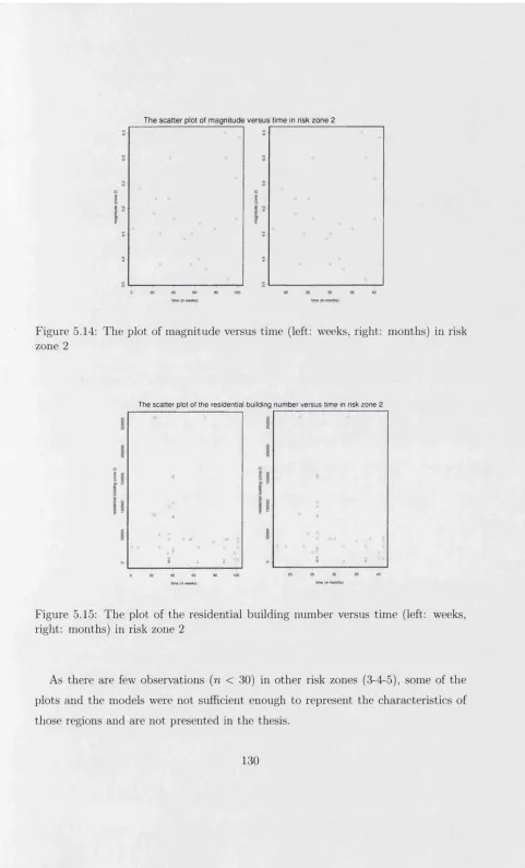
in risk zone 2 ... 129 5.14 The plot of magnitude versus time (left: weeks, right: months) in

risk zone 2 ...130 5.15 The plot of the residential building number versus time (left: weeks,

right: months) in risk zone 2 ...130 5.16 The plot of /3 selection in zone 1 versus deviance values by the expo­

nential kernel use for the number of claims m o d e l ...135 5.17 The plot of the number of claims versus time (in months) in zone 1

by the exponential kernel use ...136 5.18 The plot of the fitted values versus time (in months) in zone 1 by the

exponential kernel u s e ... 136 5.19 The plot of log number of claims versus log fitted values in zone 1 by

the exponential kernel u s e ... 137 5.20 The plot of the residuals of the number of claim model in zone 1 by

the exponential kernel u s e ... 137 5.21 The plot of the number of claims versus time (in months) in zone 2

5.22 The plot of the fitted values versus time (in months) in zone 2 by the exponential kernel u s e ... 138 5.23 The plot of log number of claims versus log fitted values in zone 2 by

the exponential kernel u s e ... 139 5.24 The plot of the residuals of the number of claim model in zone 2 by

the exponential kernel u s e ... 139 5.25 The plot of the number of claims versus time (in weeks) in zone 1 by

the exponential kernel u s e ...141 5.26 The plot of the fitted values versus time (in weeks) in zone 1 by the

exponential kernel u s e ... 141 5.27 The plot of the number of claims versus time (in weeks) in zone 2 by

the exponential kernel u s e ... 142 5.28 The plot of the fitted values versus time (in weeks) in zone 2 by the

exponential kernel u s e ... 142 5.29 The plot of the number of claims versus time (in months) in zone 1

by the power kernel u s e ... 143 5.30 The plot of the fitted values versus time (in months) in zone 1 by the

power kernel use ... 144 5.31 The plot of the number of claims versus fitted values in zone 1 by the

power kernel use ... 144 5.32 The plot of the residuals of the number of claim model in zone 1 by

the power kernel u s e ... 145 5.33 The plot of the number of claims versus time (in weeks) in zone 1 by

the power kernel u s e ... 146 5.34 The plot of the fitted values versus time (in weeks) in zone 1 by the

power kernel use ... 147 5.35 The plot of the number of claims versus time (in weeks) in zone 2 by

the power kernel u s e ... 147 5.36 The plot of the fitted values versus time (in weeks) in zone 2 by the

5.37 The plot of the claim amount versus time (in months) in zone 1 by the exponential kernel u s e ... 153 5.38 The plot of the fitted values versus time (in months) in zone 1 by the

exponential kernel u s e ... 153 5.39 The plot of the claim amount versus fitted values in zone 1 by the

exponential kernel use ... 154 5.40 The plot of the residuals in zone 1 by the exponential kernel use . . . 154 5.41 The fitted estimate of the event arrival rate A( t )...161 6.1 The plot of the claim amount versus magnitude in all risk zones (1-5) 164 6.2 The plot of the residential building number versus magnitude in all

risk zones ( 1 - 5 ) ...164 6.3 The plot of the claim amount versus magnitude in risk zone 1 . . . . 165 6.4 The plot of the residential building number versus magnitude in risk

zone 1 ...166 6.5 The plot of the claim amount versus magnitude in risk zone 2 . . . . 166 6.6 The plot of the residential building number versus magnitude in risk

zone 2 ...167 6.7 The plot of the claim amount versus residential building number in

all risk zones (1-5) 168

6.8 The plot of magnitude versus residential building number in all risk zones (1 -5 )...168 6.9 The plot of the claim amount versus residential building number in

risk zone 1 ...169 6.10 The plot of magnitude versus residential building number in risk zone 1169 6.11 The plot of the claim amount versus residential building number in

risk zone 2 ...170 6.12 The plot of magnitude versus residential building number in risk zone 2170 6.13 The scatter plot of number of claims versus magnitude in risk zone 1

6.14 The scatter plot of claim amount versus magnitude in risk zone 1 by weeks d a t a ...171 6.15 The scatter plot of number of claims versus magnitude in risk zone 2

by weeks d a t a ...172 6.16 The scatter plot of claim amount versus magnitude in risk zone 2 by

weeks d a t a ...172 6.17 The plot of the claim number versus time (in months) in risk zone 1

by the exponential kernel use ...176 6.18 The plot of the fitted values versus time (in months) in risk zone 1

by the exponential kernel use ...177 6.19 The plot of the claim number versus time (in weeks) in risk zone 1

by the exponential kernel use ...178 6.20 The plot of the fitted values versus time (in weeks) in risk zone 1 by

the exponential kernel u s e ... 178 6.21 The plot of the claim number versus time (in months) in risk zone 1

by the power kernel u s e ... 179 6.22 The plot of the fitted values versus time (in months) in risk zone 1

by the power kernel u s e ... 180 6.23 The plot of the claim number versus time (in weeks) in risk zone 1

by the power kernel u s e ... 181 6.24 The plot of the fitted values versus time (in weeks) in risk zone 1 by

the power kernel u s e ... 181 6.25 The plot of the claim number versus time (in months) in risk zone 1

by the power kernel u s e ... 184 6.26 The plot of the claim amount versus time (in months) in risk zone 1

by the power kernel use in covariate models ... 185 6.27 The plot of the fitted values versus time (in months) in risk zone 1

by the power kernel use in covariate models ...185 6.28 The plot of the claim amount versus time (in weeks) in risk zone 2

6.29 The plot of the fitted values versus time (in weeks) in risk zone 2 by the power kernel use in covariate m o d e ls ... 187 7.1 Annual reported economic damages from natural disasters:

1975-2005. Source: E M D A T ... 200 7.2 Great natural catastrophes 1950-2002... 200 7.3 The bar plot of the number of claims in risk zone 1. Left: in terms

of months, right: in terms of weeks...220 7.4 The plot of the exponential kernel function in risk zone 1. x-axis:

time (in weeks), y-axis: the exponential k e rn e l... 221 7.5 The plot of the fitted A* in risk zone 1 by exponential kernel, x-axis:

time (in weeks), y-axis: A * ...221 7.6 The exponential kernel in risk zone 1 at weeks 29, 35, 59, 74, 81 and

1 1 2 222

7.7 The plot of the aggregate mean in risk zone 1 by the use of the exponential kernel, x-axis: time (in weeks), y-axis: the aggregate mean E ( S ( t ) )... 223 7.8 The plot of the aggregate variance in risk zone 1 by the use of the

exponential kernel, x-axis: time (in weeks), y-axis: the aggregate variance V a r ( S ( t ) )... 224 7.9 The plot of the A* deviation versus time, x-axis: time (in weeks),

y-axis: the deviation of A j ...224 7.10 The plot of the exponential kernel function in risk zone 1. x-axis:

time (in weeks), y-axis: the exponential k e rn e l... 227 7.11 The plot of the fitted A* in risk zone 1 by exponential kernel, x-axis:

time (in weeks), y-axis: A * ...227 7.12 The effects of the Marmara earthquake on major macroeconomic vari­

10.4 Economic damage from natural disasters reported for 2004 ... 255 10.5 The earthquake zone map of Turkey. Source: G D D A ...255 10.6 The fault map of T u rk e y ... 256 10.7 Comparison of the North Anatolian Fault and San Andreas Fault . . 256 10.8 The ruptures in the NAF by y ears...257 10.9 Some images after the Marmara e a r th q u a k e ... 257 lO.lOSome images of the house damage after the Marmara earthquake . . . 258 lO.llHuman impact by disaster types: comparison 2004-2005. Source:

E M D A T ...258 10.12Natural disaster occurrence by disaster type: comparison 2004-2005.

Index of N otation

t , T: time.

N(t): The claim number process up to time t.

X(t): The claim amount (claim size) process up to time t. N i’.The number of claims (bin count).

Xi. The claim amount in the corresponding bin (X{ = X ti).

S f . The aggregate claim (total claim amount) in the corresponding bin.

fif. The mean of the aggregate claims 5*.

Tfi'. The mean of the raw claim amount X(.

Ti. The variance of the raw claim amount X{. A(t): The intensity (rate) of N(t) process.

A(t): The mean function (the intensity) of the whole process of N(t) (aka the expected number of events by time t). This notation is used for non-bin case.

A*: The intensity function A for binning case (also used as Ai). S(t): The aggregate claims or the total claim amount process. R(t): The risk process of a company (aka surplus).

d: The deductible amount.

/?: The non-linear parameter to represent the exponential decay (trend) in the earthquake risk zones in Turkey.

a y The coefficients representing the effect of earthquakes.

n: The number of observations (earthquake claims).

i: The index for the number of observations, i = 1, . . . , n.

k: The number of the knots to replace the kernel function for the empirical earthquakes.

j: The index for the knots to replace the kernel function for the empirical earth­ quakes, j = 1, . . . , k.

0: Vector of the intensity function A’s, which is consisted of the a and (3 param­ eters.

C hapter 1

In trod uction

The 1999 Marmara earthquake was a turn point in the earthquake research in many aspects (e.g building damage, socio-economic losses) in a highly earthquake-prone country like Turkey. The main question in people’s mind since then is ‘What hap­ pens if another earthquake strikes with a similar or bigger magnitude?’. Different scenarios are prepared to answer this question, especially for Istanbul and surround­ ings, which are situated in the earthquake risk zone 1 according to the classification of the Earthquake Region Map of Turkey (see the Appendix).

Most of the earthquake research are conducted by the civil engineers and geol­ ogists on fault structures, building structure and damage assessment, where psy­ chologists and sociologists study the social impacts of disasters. In this thesis, we wanted to contribute to all these vital studies with a financial and statistical point of view. In what way can statistics science be included in such research rather than just keeping the basic numbers like the number of the earthquakes, the number of life losses.

enough to be able to cope with the claims arriving after an earthquake.

This thesis studies the mandatory earthquake insurance claims data, which is collected in the Turkish Catastrophe Insurance Pool between December 2000 and July 2003. Chapter 2 gives information on the earthquakes, the hazard profile and earthquake history of Turkey and the most devastating earthquake of all times in the country, that is the 17/August/1999 Marmara (Kocaeli) earthquake. Chapter 3 is mainly the literature review of the distribution theory of the Poisson (homogeneous, inhomogeneous) process, the premium calculation, reinsurance, the moment gener­ ating and cumulant functions, the extreme value theory and its application to the data of this study. Chapter 4 introduces the likelihood function of the observations and time. The parameter estimates are given for Poisson likelihood of the number of claims model, iV*, and for Normal likelihood of the aggregate claims (total claim amount) S{ model since log Si ~ Normal with the use of the special functions, which are the exponential and the power kernel functions.

C hapter 2

E arthquakes

2.1

H istorical view

Earthquakes are the results of the continuous reshaping of the Earth. In time, people tried to explain the shakings, which killed many of them and caused damage to their homes and lives. People did not have any knowledge of earthquakes scientifically, so they made up some legends, stories about monsters shaking the Earth. For instance, in ancient Japan, it was believed that Namazu, a big catfish, was living underground and when Namazu moved the ground was shaken. A God, Daimyojin, would control Namazu. When Daimyojin’s attention was not on the catfish, the fish moved and that caused earthquakes. There were no answers to the questions in people’s mind except such kind of legends, until Greek philosophers, like Strabo and Aristotle thought the earthquakes were caused by something going on physically underground [Bolt, 1988].

although they are mentioned as early as 580 BC. The earliest known earthquakes in the American continent were in Mexico in the late fourteenth century and in Peru in 1471, but the records of them are not extensive. By the seventeenth century, descriptions of the effects of earthquakes started to be published around the world. In the recorded history of North America, there were a series of earthquakes, which occurred in 1811-1812 near New Madrid, Missouri. A big earthquake of magnitude 8.0 occurred on 16/December/1811. Another one occurred on 23/January/1812, and a third one, on 07/February/1812. The aftershocks of these earthquakes lasted for months [Bolt, 1988].

In 1906, one of the most destructive earthquakes throughout the recorded history of North America occurred in San Francisco. The earthquake itself and the following fires caused approximately 700 life losses and left the city in ruins. Year 2006 is the 100th anniversary of this earthquake. The Alaska earthquake of 27/March/1964 was greater than the San Francisco earthquake in magnitude, yet since the epicentre was fax from the densely populated area, only 114 people died.

It is also noticeable and interesting that earthquakes destroyed the three of the Seven Wonders of the World in ancient times: the Mausoleum of Halicarnassus, the Colossus of Rhodes and the Pharos of Alexandria.

W hat is an earthquake?

crust [Bolt, 1988, Coburn and Spence, 1992].

Scientists specify different types of earthquakes. The most well-known earthquake is a Hedonic earthquake’, which is defined above. Almost 90 % of the earthquakes are of that kind. The second one is a 1 volcanic earthquake’, which occurs as a result of volcanic eruptions with the same mechanism to change the surface structure of the Earth as in tectonic ones. Another type of an earthquake is the one, which occurs in the underground caverns and mines, where the roof of the cavern or mine collapses. It is called a ‘collapse earthquake’. Sometimes, landslides can produce earthquakes. The last type is an 1 explosion earthquake’. There are nuclear test sites around the world. When there is a detonation of nuclear and chemical devices in these sites, a big amount of nuclear energy is released and this may cause earth­ quakes [Bolt, 1988, Coburn and Spence, 1992].

How does an earthquake occur?

There are three types of waves:

P-wave : The P-wave is generated in a body of the rock and is faster than the other waves. It can move in solid rock, like granite mountains, with a speed of 6 km/sec and in liquid material, such as volcanic magma and oceans, with a speed of 2 km/sec. This characteristic of the P-wave is similar to normal sound waves. When P-waves occur, a fraction of them can be transmitted into the atmosphere like sound waves so that animals and humans can hear them. In most of the earthquakes, the P-waves are felt first.

S-wave : Being generated in a body rock like P-wave, the S-wave is slower than P- wave with a speed of 3 km/sec. It cuts the rock sideways at right angles to the direction of travel. They can not travel in the liquid areas of the Earth. Surface wave : This is so-called since its movements are always near to the ground surface. It

is like little waves, a light fretting of the surface of a liquid, as with movements on a lake. They move slower than the body (P and S) waves. There are two kinds of surface waves:

a- Love wave: The love wave moves the ground from side to side in a horizontal plane but at right angles to the direction of transmission. The horizontal movement of the love waves damages the foundations of structures. It affects only the surface water as the sides of lakes and oceans.

b- Rayleigh wave: The Rayleigh wave moves both horizontally and vertically in a vertical plane, in the direction of the transmitting waves. It moves slower than the love wave.

much safer to make construction on solid surfaces rather than sand, water-saturated soil and alluvium.

The breaking in the E arth’s crust, which can be observed as discontinuities in rock structure, is called a 1 fault'. Some of the faults ended the displacements thousands of years ago. Therefore, they are called £inactive faults'. It is the active faults, which cause earthquakes with sudden ruptures as they move very slowly by the time. Their yearly movements can be measured in millimetres. They can be both on the surface of the earth or under the sea. There are three types of faults determined by their movements: Normal, strike and reverse faults. If the fault plane moves downward by the tension, it is a ‘normal fault'. When the fault planes pass horizontally through one another, it is a ‘strike fault'. The ‘reverse' fault is where the wall of the fault moves up from the dip of the fault plane by compression. The special case of reverse fault is a 1 thrust fault', when the dip of the fault is small. Vertical displacements occur in normal and strike faults, which are called ‘dip-slip faults',

whereas the horizontal ones along the strike of the fault are called ‘strike-slips'

[Bolt, 1988, Coburn and Spence, 1992].

There is no guarantee that whenever an earthquake occurs along a fault there will not be another one in the future. There can always be some energy, which was not released by the latest earthquake. By using the results of the geological surveys, it is safer to make construction away from the fault lines. This mitigation effort can reduce the damage after the earthquakes. Furthermore, dip-slip faults can cause more damage than the strike-slip ones. It is the responsibility of the city-planners, the engineers and the central and local administration to decide where and what to build in settlement areas.

How to measure earthquakes?

For the first time, Chang Heng, a Chinese scholar, invented the device ‘seisrao-

developed at the beginning of the twentieth century. The seismograph gives us the detailed record of an earthquake from the beginning to the end. The zigzag line record is called a lseismogram\ It shows the motion of the earthquake on a mag­ netic tape either photographically or electromagnetically. The path of the P, S and surface waves can be followed by the seismograms.

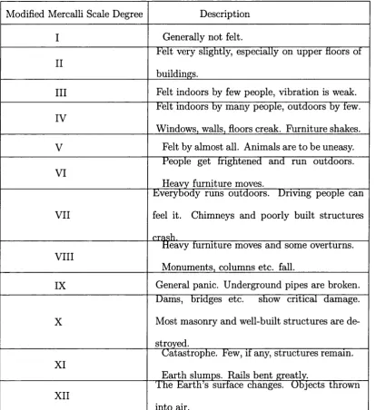
Mainly two terms are used to describe the size of earthquakes. The first one is ‘ intensity ’. Intensity measures the severity of the shaking of the ground at a specific location. By using the intensity scales developed through time, it can be guessed that how the earthquakes can affect the people and the environment. An Italian scientist, Michele Stefano de Rossi and Francois Forel of Switzerland developed the first modern intensity scale in the 1880s. Today, the Modified Mercalli (MM) Intensity Scale is one of the scales used to measure the intensity (see Table 2.2). Originally, Giuseppe Mercalli, the Italian seismologist and volcanologist constructed this scale in 1902. H. O. Wood and Frank Neumann had revised the scale in 1931. Later, in 1956, the American scientist, Charles F. Richter again revised it by using the masonry as indicator of intensity in a 12-point scale. The 12-point scale is commonly used in Unites States. The one generally used in Europe is the Medvedev- Sponheuer-Karnik (MSK) scale. In Japan, the Japanese Meteorological Agency (JMA) scale and 7-point scale in use. In China, they have their own scales related to their building types.

The other term, which many people heard of, is the ‘ magnitude of an earthquake’. The magnitude is a measure of the size of the earthquake. There are some scales to measure magnitude, like intensity scales. In 1931, K. Wadati originally prepared the most famous of them in Japan. Later, in 1935, Charles F. Richter developed one at the California Institute of Technology and it is named after him, the Richter Scale.

32-times stronger energy, which is the destructive power of the earthquakes. The earthquakes with magnitude 5.0 or more are considered to cause damage. There is a power relation, which is used to explain the effect of earthquakes with different magnitudes. Here is an example:

How much bigger is an earthquake w ith m agnitude 8.4 than the one w ith 5.2?

I Q8 -4

—— = io8-4- 5-2 = 103'2 = 1585 10

Therefore, an earthquake with magnitude 8.4 has 1585 times destructive effect than the one with magnitude 5.2. The table below gives energy information about the ef­ fects of the earthquakes with different magnitudes [Coburn and Spence, 1992] (Page

21).

Magnitude Effect

less than 4.5

An earthquake with magnitude less than 4.5 generally does not cause damage. Approxi­ mately 108 kilojoules of energy (equivalent to 10 tons of TNT exploded underground) is re­ leased in an earthquake of magnitude 4.5.

4.5-6.0

Damage generally occurs after an earthquake of magnitude 5.0. It is estimated that 109 kilojoules of energy (equivalent to 1000 tons of TNT exploded underground) is released in an earthquake of magnitude 5.5.

6.0-7.0

With magnitude 6.0, 1010 kilojoules of energy (equivalent to 6000 tons of TNT exploded un­ derground) is released. This is 1012 kilojoules for an earthquake of 7.0 magnitude.

7.0-8.9

It is terrifying that an earthquake of magni­ tude 8.0 releases 1013 kilojoules energy that is equal to the explosion of 400 atomic bombs un­ derground.

Modified Mercalli Scale Degree Description

I Generally not felt.

II

belt very slightly, especially on upper fioors of buildings.

III Felt indoors by few people, vibration is weak. IV

Felt indoors by many people, outdoors by few. Windows, walls, floors creak. Furniture shakes.

V Felt by almost all. Animals are to be uneasy.

VI

People get frightened and run outdoors. Heavy furniture moves.

VII

Everybody runs outdoors. Driving people can feel it. Chimneys and poorly built structures crash.

VIII

Heavy furniture moves and some overturns. Monuments, columns etc. fall.

IX General panic. Underground pipes are broken.

X

Dams, bridges etc. show critical damage. Most masonry and well-built structures are de­ stroyed.

XI

Catastrophe. Few, if any, structures remain. Earth slumps. Rails bent greatly.

XII

The Eartffs surface changes. Objects thrown into air.

2.2

In troduction to Turkish Earthquakes

2.2.1 H azard P rofile o f Turkey

The country profile of Turkey is sourced from the CIA Country Factbook.

Total area: 780,580 sq km

Total population: 70,413,958 (July 2006 estimate)

GDP purchasing power parity: 572 USDb (2005 estimate)

GDP per capita: 8,200 USD (2005 estimate)

Unemployment rate: 10 % (plus underemployment of 4.0 %) (2005 estimate)

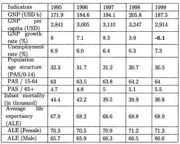
Table 2.3 summarises some social and economical indicators of Turkey. It is observed that the Gross National Product (GNP) growth rate drastically hits a negative value in 1999 (-6.1) due to the effect of the 1999 earthquakes.

Indicators 1995 1996 1997 1998 1999

GNP (USD b) 171.9 184.6 194.1 205.8 187.5

GNP per

capita (USD) 2,841 3,005 3,110 3,247 2,914

GNP growth

rate (%) 8 7.1 8.3 3.9 -6.1

U nemployment

rate (%) 6.9 6.0 6.4 6.3 7.3

Population age structure (PAS/0-14)

32.3 31.7 31.2 30.7 30.5

PAS / 15-64 63 63.5 63.8 64.2 64

PAS / 65+ 4.7 4.8 5 5.1 5.5

Infant mortality

(in thousand) 44.4 42.2 39.5 38.9 36.8

Average life expectancy (ALE)

67.9 68.2 68.6 68.8 68.9

ALE (Female) 70.3 70.5 70.9 71.2 71.3

ALE (Male) 65.7 65.9 66.3 66.5 66.6

The United Nations Development Programme (UNDP) announces Turkey as the third country after Iran and Yemen according to the number of deaths as a result of earthquakes. Earthquakes are the types of disasters, which occur with low frequency but high severity. The UNDP also ranks Turkey 35th among fifty five countries for the flood losses. In [Gurenko et al., 2006], the number of fatal earthquakes occurred in Turkey during the twentieth century is reported as 111 with total fatalities of 99,391. Floods, rock-falls, landslides and avalanches are the other types of disasters that the country faces (see the Appendix), where floods and landslides are mainly experienced in the Black Sea Region and the coastal areas. Table 2.4 gives the figures of different types of natural disasters in Turkey since 1990.

Event Date Killed Injured Homeless Affected Loss in _{$ m}

Earthquake

(Erzincan) 13/03/1992 653 3,850 95,000 250,000 750

Avalanches (S. Anatolia)

1992 (14

events) 328 53 11,600 30,000 25

Avalanches (S.& E. Anatolia)

1993 (31

events) 135 95 1,100 300 10

Mud flood (Senirkent-Isparta)

13/07/1995 74 46 2,000 10,000 ₆₅

Earthquake

(Dinar) 01/10/1995 94 240 40,000 120,000 100

Flood (Izmir) 04/11/1995 63 117 6,500 300,000 1,000

Earthquake (Qorum-Amasya)

14/08/1996 0 6 9,000 17,000 30

Flood (W.

Black Sea) 21/05/1998 10 47 40,000 1,200,000 1,000

Earthquake

(Ceyhan) 27/06/1998 145 1,600 88,000 1,500,000 500

Earthquake

(Marmara) 17/08/1999 17,480 43,953 675,000 15,000,000 16,000

Earthquake

(Diizce) 12/11/1999 763 4,948 35,000 600,000 750

Earthquake

(Sultandagi) 03/02/2002 42 327 30,000 222,000 95

Earthquake

(Bingol) 01/05/2003 177 520 45,000 245,000 135

Total 19,964 ” 55^802 l,07S;20t 19,494,300 20,460

Table 2.5 is compiled from the data of the General Directorate of Disaster Affairs and the Project Implementation Unit of the Prime Ministry Turkey and gives the type of the disaster and the related building collapse since the beginning of the twentieth century.

The type of the disaster 1 he number ot collapsed buildings

Earthquake 612,000

Landslide 65,551

Flood 61,000

Rockfall 30,000

Avalanche 5,500

Total 774,051

Table 2.5: The types of the disasters in Turkey and resulting building collapse between 1900-2003. Source: GDDA, PIU

2.2.2

T h e H isto r y o f E arthquakes in Turkey

Turkey is a peninsula, which is a bridge between the continents of Europe and Asia. The country is one of the most earthquake-prone countries in the world with 96 % of the total land, 98 % of the total population, 90 % of the cities, 755 industrial complexes and 40 % of the dams being situated in the active zones [Ozerdem and Barakat, 2000]. An Earthquake Region Map (see the Appendix), which divides Turkey into five risk zones, has been published in 1996 by the General Directorate of Disaster Affairs, Ministry of Public Works and Settlement. This map shows that 66 % of land area of Turkey is located in risk zones 1 and 2, where 70

% of the total population live in and 69 % of the industrial facilities are located. After the 1999 earthquakes, the Earthquake Map of Turkey is being revised by the scientists since the fault structures changed significantly.

of the Alpine-Himalayan fault line, which restricts the Arabian-Eurosian tectonic plates. Many studies have been carried out to understand the structure and the behaviour of the North Anatolian fault. The fault line starts in Karliova-Bingol in Eastern Turkey and continues to the west of the Marmara region with a length of 1000 kilometers. It separates North Anatolia from Middle Anatolia. The most important earthquakes in the history of the Anatolian Peninsula were due to the ruptures in the North Anatolian fault. The NAF has some similarities with the San Andreas fault, which is the cause of the 1994 Northridge earthquake, California, in movement (both from east to west), slip rate, age, length and straightness (see the Appendix) [KOERI, 1999, Bibbee et al., 2000, Erdik, 2000].

The 1939 Erzincan earthquake is the start of the chain of earthquakes along the North Anatolian fault. Between 1939-1944, the fault was ruptured 600 kilometers to the west. Afterwards, this movement slowed down and another rupture of 100 kilo­ meters was recorded between 1957-1967. The 1999 Marmara and Diizce earthquakes filled the 100-150 kilometers gap of the previous ruptures [Bibbee et al., 2000].

Magnitude 1900-1932 1933-1966 1967-2004

8.0-9.9 0 0 0

7.0-7.9 3 13 5

6.0-6.9 6 14 18

5.0-5.9 6 28 27

Total 15 55 50

Total number of

estimated deaths 4,926 48,410 28,522

Table 2.6: The significant earthquakes in Turkey between 1900-2004. Source: The General Directorate of Disaster Affairs (GDDA)

[Erdik, 2003]. It is estimated that there will be 70,000 life losses, 520,000 injuries (400,000 of which is heavy) and a direct economic loss of USD 30b [Erdik, 2003].

2.3

1 7 /A u g u st/1 9 9 9 M arm ara (K ocaeli) E arth­

quake

On 17/August/1999, at 03:01:37 a.m. local time, one of the most devastating earth­ quakes in the history of Turkey occurred as a result of the 120-kilometre rupture of the North Anatolian fault near Akyazi-Yalova region and lasted approximately 45 seconds. The epicentre was in 18 kilometres (10.5 miles) depth near to Golciik, the town 11 kilometres (7 miles) to the southeast of the city of Izmit (Kocaeli) where the country’s main naval base is located. The magnitude of the earthquake was 7.4 in Richter Scale and caused 2.7 metres (9 feet) right-lateral strike-slip movement on the fault. Preliminary field reports confirm this type of motion on the fault, and initial field observations indicate that the earthquake produced at least 60 kilome­ tres (37 miles) of surface rupture. The more specific magnitude measurements are given below:

Surface Wave Magnitude: 7.8 (U.S. Geological Survey-USGS)

Body Wave Magnitude: 6.3 (USGS)

Duration Magnitude: 6.7 (Bogazigi University Kandilli Observatory and Earthquake Research Institute)

Moment Magnitude: 7.4 (USGS, Kandilli Observatory and Earthquake Research Institute)

Epicentre: 40.702N, 29.987E (USGS)

Depth: 18 km. (USGS)

% of industrial value added. Together with the other affected, surrounding cities (Istanbul, Bursa, Eskisehir) in the region, those values increase to 34.7 % and 46.7 %, respectively [Erdik, 2000]. The Marmara Region counts for the 5 % of export and 15 % of import trade of Turkey. The per capita income of the region is the double of the national average [SPO, 1999].

The earthquake caused almost 18,000 deaths and 45,000 injured th at approxi­ mately 20,000 of the injured were left permanently disabled. Small coastal towns (e.g. Degirmendere, Golciik) were severely affected by the earthquake. Apart from the earthquake itself, tsunamis (tidal waves due to the sea floor earthquakes) hit the towns. Since it was summer time, the population of the coast towns was higher than that of in winter. Many were killed when they were asleep. There are no confirmed records on the losses caused by tsunamis.

M onetary losses:

Industrial facilities: USD 2b (most of them insured with an insured value of USD 15b)

Buildings: USD 5b (about 8 % insurance penetration)

Railways'. USD lb

Highways’. USD 0.2b

Ports: USD 0.2b

Telecommunication: USD 75m

Energy transmission: USD 3m

Average total losses (physical and socio-economic): USD 16-20b (approximately 7-9

% of the GDP).

The damage to industry was estimated at USD 1.1 - 4.5b by the public and private sectors. The added-value loss stemming from that is about USD 700m, which results in a 1.6 % decrease in the growth of the production sector. The payments of the claims are to be estimated around USD 600-800m since most of the industry losses were covered by insurance [Erdik, 2000, SPO, 1999].

Farge). The State Planning Organisation (SPO) estimates a total loss of USD 880m for the state-owned ones (Tiipra§, Tuvasa§, Igsa§, Petkim, Seka and Asil Qelik).

It is also estimated by the State Planning Organisation that there is a burden of USD 6.2b on public finance caused by the earthquake. USD 3.5b of this amount is used for the reconstruction of houses after the disaster. The government enacted special earthquake taxes and allowed a paid military service for men between certain ages, which have not yet done their military service for various reasons. A year after the earthquake, USD 3b was obtained by these temporary solutions. International resources like the European Union and the World Bank supplied USD 2.5b for the reconstruction and recovery period. There was a 5 % decline in the GDP during 1999, which was stopped in the first half of 2000. By the August 2000 report of the SPO, a 5 % increase in annual GDP was realised [Selguk and Yeldan, 2001].

Apart from all the economic losses briefly summarised above, there are some psychological effects of the earthquake which will take a long time to recover. People lost their families, homes and jobs. As a result, there has been a high increase in suicide, depression, alcohol consumption, problems in the families and the divorce rate. Most people do not want to get married on the 17th August and do not celebrate birthdays on that day.

The damage reports show that most of the collapsed and heavily damaged build­ ings were 6-8 storey, some were under construction and some were built within last few years before the earthquake. In Turkey, there is a current Building Code of 1998 with necessary regulations for sophisticated earthquake-resistant buildings. This code is an adaptation of the Californian Uniform Building Code to the stan­ dards of Turkey. Although those damaged and collapsed multistorey buildings are supposed to be earthquake-resistant, they were not due to the following factors [Giilkan, 2000]:

1. Inadequate vertical and horizontal reinforcing steel and the widespread use of smooth (as opposed to deformed) reinforcing steel,

the construction,

3. The use of poor and inappropriate materials in construction, 4. Poor workmanship,

5. Allowance to make construction on active faults and in areas of high liquefac­ tion potential,

6. The use of past experience instead of the engineering techniques to make buildings.

Building damage statistics after the Marmara earthquake are given in Table 2.7 below.

Number of housing units Number of business premises

Total collapse-destroyed 66,441 10,901

Moderate damage 67,242 9,927

Light damage 80,160 9,712

Total 213,843 30,540

Table 2.7: The building damage after 1999 Marmara earthquake. Source: Govern­ ment Crisis Centre, [Bibbee et al., 2000]

Earthquake Protection and Preparedness

Earthquake itself, following fires, landslides, mudslides, avalanches, tsunamis, se­ iches, floods from dams and soil liquefaction are the important factors, which cause casualties and damages and increase the total losses. It is possible to reduce the losses of earthquakes by some mitigation methods and effective disaster risk pre­ paredness and management plan. The following are some basic steps for individuals to do before, during and after an earthquake [Bolt, 1988]:

1. Before an earthquake:

i) Have a flash-light and a first-aid kit in your home. Each household should know where they are kept.

ii) Learn first-aid.

iii) Do not keep heavy objects on the shelves. 2. During an earthquake:

i) Keep calm. Stay wherever you are, indoors or outdoors. A large number of deaths are due to the heart attacks and jumping from balconies or windows due to panic.

ii) If near to an exit or can reach to exit easily, leave the building as soon as possible. Do not stay to collect belongings and valuables.

iii) If indoors (upstairs), stand against a wall near the centre of the building. Do not get close to the windows, balconies and outdoors. Do not try to run away through the elevators or stairs. If possible, stay close to heavy furniture like washing machine or dishwasher since they can provide a space for you to survive until the rescue teams reach.

iv) If outdoors, stay in the open. Keep away from overhead electric wires or anything that may fall.

vi) If you are in a moving car, stop away from the overpasses and bridges and remain inside the car until the shaking stops.

3. After an earthquake:

i) Check yourself and others nearby for injuries. Provide first-aid if needed. ii) Check water, gas and electric lines. If damaged, close the valves.

iii) Check for gas leaks. If detected, open all the windows and outdoors, leave immediately and report it to the authorities.

iv) Turn on the radio for emergency instructions. Do not keep the telephone lines busy as there may be some urgent calls.

v) Stay out of damaged buildings.

vi) Do not use lifting machinery, bulldozers or mechanical diggers to move the rubble even if they are available. It is highly possible survivors could be killed under the rubble if you use them. Use manual labour.

vii) Think of where people could be trapped under the rubble. Listen for people inside the rubble replying or making noise for help.

C hapter 3

D istrib u tion T heory

In this chapter, the available literature is revised on the claim number process, the claim arrival times, the total claim amount (the aggregate claims) process, the use of the aggregate claims in the actuarial context, the moment generating functions and the application of the extreme value theory with the use of extreme events data.

3.1

P oisson P rocess

3.1.1

H om ogen eou s and In h o m o g en eo u s P o isso n P ro c ess

The claim number process is a stochastic process, which has a very wide use in the insurance and actuarial studies in estimating the risk process of a company. Let N(t) be the process of the number of claims in the interval (0,t]. In classical risk theory, the claim number process is generally assumed to have independent increments. If the intensity A of claim frequency is independent of time t, then

N(t) is a homogeneous Poisson process with intensity A > 0 [Biihlmann, 1970, Cox and Miller, 1965, Rolski et al., 1999]. Then the probability density function of the distribution of N(t) is Poisson

Pr{N{t) = n) = — ---- (n = 0 ,1 ,2 ...),

2. For any time points to = 0 < ti < < ... < tn, the process increments

N(t\) — iV(to), -/V(t2) — N ( t i) , . . . , N( t n) — N ( t n-1) are independent Poisson random variables and stationary (i.e. all increments of intervals of the same length have the same distribution).

The moments of the claim number process N(t) are given as follows by using the properties of the Poisson distribution (mean=variance)

E(N(t)) = At,

and

Var(N(t)) = At.

The claim number process N(t) is assumed to be a counting process with random time

tn = IVi + ... + Wn {n > 1).

The differences tn = Wn+1 — Wn are called event (claim) interoccurrence (inter- arrival) time. Any counting process generated by an independent identically dis­ tributed sum process tn is also called as a renewal counting process. Since a Poisson process restarts itself at any point in time, there is no memory of the past (renewal) and this differs the Poisson process from other renewal processes.

One can also define N(t) as a pure jump process with sample paths in Z)[0, oo) that increase to oo as t —► oo with jumps of height 1 at the random times t n. Since any process with independent, stationary increments and simple paths in D[0, oo) is a Levy process, N(t) satisfies this definition and also entitled to be a Levy process. By all of the properties it has, the claim number process N(t) is [Embrechts et al., 1997]:

1. A homogenous Poisson process, 2. A renewal process,

The rate A in a Poisson process N(t) is the proportionality constant in the prob­ ability of an event occurring during an arbitrarily small interval. It is relevant to consider the rate A as time varying, that is A = A(t), in many applications. In that case, the process N ( t) is an inhomogeneous (non-homogeneous) or non-stationary

with time. When N(t) is an inhomogeneous Poisson process with rate A(£) (gener­ alisation of a Poisson Process), then the increment N(t) — N (0), given the number of events in an interval (0, t], has a Poisson distribution with parameter F^A^t)] = A0(£) = fg X(r)dr and the increments over disjoint intervals are independent ran­ dom variables [Cox and Miller, 1965, Cinlar, 1975, Daley and Vere-Jones, 2003]. In other words, the intensity A is replaced by a mean value function (or the cumulative intensity function) A(t) and N(t) is said to be an inhomogenous Poisson process with the mean value function A(t). This is called the Cox or doubly stochastic Pois­ son process, when A(t) is itself random [Biihlmann, 1970, Basu and Dassios, 2002, Ruggeri and Sivaganesan, 2002, Ruggeri et al., 2000, Ruggeri and Pievatolo, 2002, Rolski et al., 1999]. An inhomogeneous Poisson process allows some events to occur more likely at certain times than during other times [Ross, 2003, Cox and Lewis, 1966, Lewis, 1972].

When one uses the real data on the number of claims arriving in a certain time interval, it is not always suitable to use the Poisson assumption. In many cases, negative binomial distribution is preferred, which can be obtained by mixing the Poisson distribution with a gamma distribution (mixed Poisson process). In the claim arrival processes, more variability is expected. In a mixed Poisson process, this variability decreases as time goes by. By a similar argument above, to stop the decrease in the variability, Cox processes are used with the cumulative intensity measure A(a, 6] = \(r)dr (aka integrated rate function). One example of the mixed Poisson processes is the mixture of a Poisson process and Gamma distribution, which is also known as ‘Polya’ or ‘Pascal’ process.

R em ark 2: The time-dependent intensity A(t) of an inhomogeneous Poisson process N(t) is approximated by A(t) as an expansion form by the integral over A(t)

[Vere-Jones and Ozaki, 1982, Cox and Miller, 1965]. Therefore N(t) ~ Poisson(A(t)). This implies [Daykin et al., 1994b]:

1. E(N(t )) = A(t),

2. Var(N(t)) = A(t) —► standard deviation = \/A(£), 3. j ( N( t ) ) = , where 7 stands for the skewness, 4. 72(Af(t)) = where 72 stands for the kurtosis.

The use of the intensity A(t) in modelling chapters of this thesis will be based on the Poisson binning approach. That is, the rate A(t) is assumed to be a constant over each bin, which tells us that the Poisson count for the bin is equal to A(t) = $^\{r)d r, where A represents the expected number of events by time t.

R e m a rk 3: By Remark 1, if f* X(r)dr = A(b) — A(a) holds, it implies that A(r) is the intensity function of A.

R e m a rk 4: An important property of an inhomogeneous Poisson process is the additivity property of the intensities of the two independent inhomogeneous Poisson processes. This applies and easily proved for the case of regular Poisson distribution. It states in [Rolski et al., 1999] that suppose Ni(t) and N 2(t) are two independent inhomogeneous Poisson processes with intensity functions Xi(t) and A2(£), respectively. The superposition N(t), where N(t) = Ni(t) + N2(t) is an inhomogeneous Poisson process with intensity function A(t) = Ai(t) + X2(t).

Let Wo be the time of the first claim event to occur in (0, t] and N(t) be an inhomogeneous Poisson process with intensity A. Then

and

p « (1 — X(r)dr)(l — X(r)dr) . .. (1 — A(r)dr) « ^1 — A(r)dr^j t

t

t t

by using log(l — x) = — x + o(x2), where o is a function of x,

logp « — / X(r)dr

p « e - S £ x(r)d r?

and the cumulative distribution function is

Fo( 0 = P r(W 0 < t ) = l - Pr(W o > 0 = 1 - e - l o A(r)*

As explained in [Biihlmann, 1970], Markov processes are the generalisation of the processes with independent increments. Since the process above is Markovian, the times W i,W2-.. form a renewal (inhomogeneous Poisson) process and we can, by a similar argument to the above, show that conditional on Wi, the distribution of the time to the next claim event, U = Wi+i — has the following distribution function [Cox and Lewis, 1966]

and by differentiation, the probability density function is [Cox and Lewis, 1966]:

In the modelling chapters of this thesis, special kernel functions will be used: the exponential and the power kernel functions. It might be interesting to search for the type of the distribution of the first event occurrence time, fo(t), for these kernel choices before we continue with the total claim amount process. The exponential and the power kernel functions simply have the following forms, respectively: where

(3.1)

and

log A(£) = a t13.

If the exponential kernel is substituted in fo(t) with A(t) = eae Pt, we have

/ „ ( * ) = e a e - « e - /0‘ e » '- 'S‘ dr

The question arises here is to find the recognisable distribution of this form. For

(3 = 1, the exponential kernel takes the form log A(t) — and this implies A(t) = eae \ By the same argument above

f 0(t) = eae~‘e - t t ‘°'~'dT.

If the integral above is solved, we have e“e and this might suggest the dis-tribution of the first event occurrence time by the use of the exponential kernel function.

When (3 = 1, the use of the power kernel results in a familiar distributional form. That is, for /? = 1, logA(t) = a t, which is log-linear case itself and A(t) = eat.

Therefore

f 0(t) = eaie - t i eQtdr = eate~eaH = eate~teat.

Let y = e*, then logy = t with the Jacobian | ^ | = |A|. Then, the distribution of the occurrence of first event with the use of the power kernel is

f y ( y ) = \ ~ \ y ay ~ ya i

which is a form of Weibull distribution. If Y ~ Weibull then log Y ~ logWeibull (aka the Fisher-Tippett distribution) appears as a distribution of the occurrence of first event with the use of the power kernel by log y = t transformation.

This will not cause a big gap in the analysis, since we use the + part of the ti — Sj

difference (in notation (ti — Sj)|+), where we never have U = Sj case (please note the use of U for the actual event, Sj to represent the site of the kernel knot).

3.2

T he to ta l claim am ount (aggregate claim s)

process

In the insurance context, the total claim amount process, S( t), has a very wide use. In this process, the claim amount X i, which corresponds to each policy, is summed up over a given time period. The calculation of S(t) depends on the claim size (amount)

Xi and the claim number process N(t) in a given time period and that leads to the calculation of the net (pure) premium [Embrechts et al., 1997, Biihlmann, 1970]. A claim is called ‘large’, when it consumes a large portion of the total claim amount [Rolski et al., 1999].

When the claim amount distributions are independent but not necessarily iden­ tical, the total claim amount process is called as the ‘individual modeV. The aggre­ gate claims model, which is often used to approximate the individual claims model [Kaas et al., 2001], is called the ‘collective modeV [Rolski et al., 1999] and defined with the following equation, assuming that the claim size X j’s and the claim number process N(t) are independent and also X^ s are independently identically distributed (i-i-d)

JV(t)

s ( t ) = j 2 X i

(*^°)>

Z = 1 where S(t) = 0 if N(t) = 0.

In the collective risk model, the insurance portfolio is thought to be a process, which generates claims over time [Kaas et al., 2001]. In both the individual and collective models, the total claims on a portfolio of insurance contracts is the random variable of interest [Kaas et al., 2001]. The total claim amount S(t) is a random variable, when the claim number process N(t) and the claim amo