comm
en
t
re
v
ie
w
s
re
ports
de
p
o
si
te
d r
e
sea
rch
refer
e
e
d
re
sear
ch
interacti
o
ns
inf
ormation
Multiclass classification of microarray data with repeated
measurements: application to cancer
Ka Yee Yeung and Roger E Bumgarner
Address: Department of Microbiology, Box 358070, University of Washington, Seattle, WA 98195, USA.
Correspondence: Ka Yee Yeung. E-mail: [email protected]. Roger E Bumgarner. E-mail: [email protected]
© 2003 Yeung and Bumgarner; licensee BioMed Central Ltd. This is an Open Access article: verbatim copying and redistribution of this article are permitted in all media for any purpose, provided this notice is preserved along with the article's original URL.
Multiclass classification of microarray data with repeated measurements: application to cancer
Prediction of the diagnostic category of a tissue sample from its gene-expression profile and selection of relevant genes for class prediction have important applications in cancer research. We have developed the uncorrelated shrunken centroid (USC) and error-weighted, uncor-related shrunken centroid (EWUSC) algorithms that are applicable to microarray data with any number of classes. We show that removing highly correlated genes typically improves classification results using a small set of genes.
Abstract
Prediction of the diagnostic category of a tissue sample from its gene-expression profile and selection of relevant genes for class prediction have important applications in cancer research. We have developed the uncorrelated shrunken centroid (USC) and error-weighted, uncorrelated shrunken centroid (EWUSC) algorithms that are applicable to microarray data with any number of classes. We show that removing highly correlated genes typically improves classification results using a small set of genes.
Rationale
The problem of predicting the diagnostic category of a given tissue sample is of fundamental clinical importance. Conven-tional diagnostic methods are based on subjective evaluation of the morphological appearance of the tissue sample, which requires a visible phenotype and a trained pathologist to interpret the view. In some cases the class is easily identified by cell morphology or cell-type distribution, but in many cases apparently similar pathologies can lead to very different clinical outcomes. Since the advent of DNA array technology [1-6], researchers have begun to use expression array analysis as a quantitative phenotyping tool. The potential advantage to using arrays for phenotyping is that they provide a simultane-ous quantitative measure of thsimultane-ousands of parameters (for example, gene-expression levels) some of which are likely to have disease relevance. When array analysis is used predom-inately for phenotyping, we refer to the expression pattern as an 'expression array phenotype'. Owing to the ability to quan-tify a large number of parameters, the use of expression array in phenotyping promises both more accurate class prediction and the identification of subclasses that could not be defined by traditional methods.
There has been a recent explosion in the use of expression array phenotyping for identification and/or classification in a variety of diagnostic areas. Examples of diagnostic categories (or classes) include cancer versus non-cancer [7,8], different subtypes of tumor [9-13], and prediction of responses to var-ious drugs or cancer prognosis [14-16]. The prediction of the diagnostic category of a tissue sample from its expression array phenotype given the availability of similar data from tis-sues in identified categories is known as classification (or supervised learning). A challenge in predicting diagnostic cat-egories using microarray data is that the number of genes is usually significantly greater than the number of tissue sam-ples available, and only a subset of the genes is relevant in dis-tinguishing different classes. Selection of relevant genes for classification is known as feature selection. This has three main applications: first, the classification accuracy is often improved using a subset instead of the entire set of genes; sec-ond, a small set of relevant genes is convenient for developing diagnostic tests; and third, these genes may lead to biologi-cally interesting insights that are characteristic of the classes of interest.
Published: 24 November 2003 Genome Biology 2003, 4:R83
Received: 4 June 2003 Revised: 14 August 2003 Accepted: 17 October 2003 The electronic version of this article is the complete one and can be
There have been many reports that address the classification and feature-selection problems, for example [9,10,14,17]. However, many of these methods are tailored towards binary classification in which there are only two classes [9,14]. More-over, there has been very limited effort to develop classifica-tion and feature-selecclassifica-tion algorithms for microarray data with repeated measurements or error estimates. Array data is well known to be noisy; for example, Lee et al. [18] showed that any single microarray output is subject to substantial variability. This is particularly true for genes with low expres-sion levels, which are more difficult to measure than genes with high expression levels. As the cost of microarray experi-ments is declining, more research laboratories are generating microarray data with repeated measurements [9,14,19,20]. Repeated measurements not only provide improved mates of gene-expression levels but can also be used to esti-mate the uncertainty or variability in the measurement. In some cases the repeated measurements are biological repli-cates (for example, independent samples), whereas in other cases only technical replicates are available. Regardless of the source, however, variability estimates should be taken into account in both clustering and classification algorithms, as variability estimates can potentially be exploited to improve the results.
We have developed two algorithms called the uncorrelated shrunken centroid (USC) algorithm, and the error-weighted, uncorrelated shrunken centroid (EWUSC) algorithm. Both USC and EWUSC are integrated feature-selection and classi-fication algorithms that are applicable to data with any number of classes. Our primary contribution is that both USC and EWUSC exploit interdependence between genes to reduce the number of selected features. In addition, EWUSC takes advantage of variability estimates over repeated meas-urements to down-weight noisy genes and noisy experiments so that no ad hoc filtering step is necessary. On the other hand, USC is applicable to microarray datasets with or with-out repeated measurements.
Introduction to classification and feature selection Classification is a supervised learning approach, in which the classes (or labels) of a subset of samples are inputs to the algo-rithm. This is in contrast to clustering, which is an unsuper-vised approach, in which no knowledge of the samples is assumed. A training set is a set of samples for which the classes are known. A test set is a set of samples for which the classes are assumed to be unknown to the algorithm, and the goal is to predict which classes these samples belong to. The first step in classification is to build a 'classifier' using the given training set, and the second step is to use the classifier to predict the classes of the test set.
In the context of gene-expression data, the samples are usu-ally the experiments, and the classes (or labels) are usuusu-ally different types of tissue samples (for example, cancer versus non-cancer, different tumor types, rate of disease
progression, and response to therapy). A typical microarray dataset consists of thousands to tens of thousands of genes, and dozens to hundreds of experiments. One challenge of classification using microarray data is that the number of genes is significantly greater than the number of samples. In this situation, it is possible to find both random and biologi-cally relevant correlations of gene behavior with sample type. To protect against spurious results, the goal is to identify the smallest possible subset of genes that correlate most strongly with the known class labels. In addition, a small subset of genes is desirable for the development of expression-based diagnostics. The problem of selecting relevant genes (or fea-tures) for classification is known as feature selection.
Cross validation is a well-established technique used to opti-mize the parameters or features chosen in a classifier. In m-fold cross-validation, the training set is randomly divided into m disjoint subsets with roughly equal size. Each of these m subsets is left out in turn for evaluation, and the other (m - 1) subsets are used as inputs to the classification algorithm. In this work, we randomly divide each class into m disjoint sub-sets (where m is less than the size of the smallest class in the training set), so that each class is represented in the subset fed to the classification algorithm. The left-out subset of the training set is used to evaluate classification accuracy because the classes of this subset are known. The most popular form of cross-validation is leave-one-out cross-validation (LOOCV), in which m is equal to the number of samples in the training set, and each sample in the training set is left out in turn to evaluate the prediction results.
Related work
van't Veer et al. [14] recently applied a binary classification algorithm to cDNA array data with repeated measurements, and classified breast cancer patients into good and poor prog-nosis groups. Their classification algorithm consists of the following steps. The first step is filtering, in which only genes with both small error estimates and significant regulation rel-ative to a reference pool of samples from all patients are cho-sen. The second step consists of identifying a set of genes whose behaviour is highly correlated with the two sample types (for example, upregulated in one sample type but down-regulated in the other). These genes are rank-ordered so that genes with the highest magnitudes of correlation with the sample types have top ranks. In the third step, the set of rele-vant genes is optimized by sequentially adding genes with top-ranked correlation from the second step. Leave-one-out cross-validation is used to evaluate and choose an optimal set of features. van't Veer et al.'s approach takes variability esti-mates of repeated measurements into consideration by using error-weighted correlation in their method. However, this method involves an ad hoc filtering step and does not gener-alize to more than two classes.
comm
en
t
re
v
ie
w
s
re
ports
refer
e
e
d
re
sear
ch
de
p
o
si
te
d r
e
se
a
rch
interacti
o
ns
inf
o
rmation
classification problem. They showed that the one-versus-all approach of combining SVM yields the minimum number of classification errors on their Affymetrix data with 14 tumor types. The one-versus-all combination approach builds k (the number of classes) binary classifiers, each of which distin-guishes one class from all the other classes. Suppose binary classifier i predicts a discriminant value fi(x) for a given sam-ple x in the test set. The combined multiclass classifier assigns sample x to the class for which the corresponding binary clas-sifier produces the highest discriminant value. In addition to not taking variability estimates of repeated measurements into account, this approach selects different relevant features (genes) for each binary classifier.
Nguyen and Rocke [21,22] used partial least squares (PLS) for feature selection, together with traditional classification algo-rithms such as logistic discrimination and quadratic discrim-ination to classify multiple tumor types from microarray data. These traditional classification algorithms require the number of samples (experiments) to be greater than the number of variables (genes), and it is therefore essential to reduce the dimensionality before applying these traditional classification techniques. PLS is a dimension-reduction tech-nique that maximizes the covariance between the classes and a linear combination of the genes. This approach can be gen-eralized to multiple classes, but it does not make use of varia-bility estimates of the data. In addition, it is a multistep process that involves a filtering step (to select genes with sig-nificant mean differences) and then application of PLS to fur-ther reduce the dimensionality so that the number of samples is greater than the number of dimensions.
Dudoit et al. [23] compared the performance of different dis-crimination methods (including nearest neighbor classifiers, linear discriminant analysis and classification trees) for clas-sifying multiple tumor types using gene-expression data. None of the discrimination methods they evaluated takes measurement variability into consideration, and their emphasis is on discrimination methods and not feature selection.
Yeung et al. [24] showed that clustering algorithms that take advantage of repeated measurements (including the error-weighted approach that down-weights noisy measurements) yield more accurate and more stable clusters. Here, we will focus on the supervised learning approach, instead of the unsupervised clustering technique.
Tibshirani et al. [17] developed a 'shrunken centroid' (SC) algorithm for classifying multiple cancer types. It is an inte-grated approach for feature selection and classification. Fea-tures are selected by considering one gene at a time: the difference between the class centroid (average expression level or ratio within a class) of a gene and the overall centroid (average expression level or ratio over all classes) of a gene is compared to the within-class standard deviation plus a
'shrinkage threshold' which is fixed for all genes. The intui-tion is that genes with at least one class centroid that is signif-icantly different from the overall centroid are selected as relevant genes. The size of the shrinkage threshold is deter-mined by cross-validation on the training set to minimize classification errors.
Our contributions
Our algorithms have the following desirable characteristics. Both EWUSC and USC exploit the interdependence of genes to reduce the number of selected features. EWUSC takes advantage of the variability of gene-expression data over repeated measurements, so no ad hoc filtering step is neces-sary. Both EWUSC and USC can be applied to data with any number of classes. Both EWUSC and USC adopt an inte-grated approach for both feature selection and classifica-tion. Both algorithms make no assumption on data distributions.
We illustrate the advantage of removing correlated genes (for example, the USC algorithm) on the NCI 60 data [12] for which there is no variability information. This dataset has been extensively used in other publications for classification algorithm development [22,23,25]. We illustrated and com-pared our USC and EWUSC algorithms with two real data-sets: a multiple tumor dataset from Ramaswamy et al. [10] and a breast cancer dataset from van 't Veer et al. [14]. These two datasets were chosen as they are publicly available in a form from which we can calculate or obtain error estimates for each gene-expression level or ratio. We used a subset of the multiple tumor data [10] that consists of 7,129 genes and 11 tumor types on Affymetrix chips. There are 96 samples in the training set, and 27 samples in the test set. For the Affymetrix dataset we estimated the variability in the gene-expression levels using the robust multi-array analysis (RMA) tool [26,27] from the BioConductor project [28]. A subset of the published data was used as we could only obtain raw data (.cel files) for a subset. The breast cancer dataset [14] consists of 25,000 genes with four repeated measurements on cDNA arrays. There are 78 samples in the training set, 19 samples in the test set, and two classes of patients: one class with good prognosis (with more than 5 years of survival time), and another class with poor prognosis (with less than 5 years of survival time). For the breast cancer cDNA array data, pub-lished p-values as calculated by Rosetta's Resolver software were used to calculate the error estimates. In addition, we cre-ated synthetic datasets with repecre-ated measurements and compared the performance of EWUSC, USC and SC at differ-ent noise levels.
is the level of agreement of selected genes chosen over differ-ent cross-validation runs of the algorithm.
Using these algorithms we obtained the following general results. Exploiting gene interdependence by removal of corre-lated genes typically results in comparable or higher predic-tion accuracy using fewer relevant genes. This is highly desirable if one wishes to develop diagnostic tools from the selected set of genes. Using error or variability estimates as weighting factors generally yields higher feature stability and reduces the number of relevant genes on real datasets. On the multiple tumor data, our EWUSC algorithm achieves 16% increase in prediction accuracy, using only 10% of the genes as features (compared with using all the available genes in the published result). On the breast cancer data, our EWUSC algorithm produces the same number of classification errors as the published result using a larger feature set. Unlike the published algorithm for this dataset, however, the EWUSC algorithm is applicable to datasets with more than two classes.
Our integrated classification and
feature-selection algorithm
As our USC and EWUSC algorithms are motivated by the shrunken centroid (SC) algorithm [17], we will briefly review the SC algorithm, and then discuss our USC and EWUSC algorithms. Details of these algorithms can be found later in the paper.
The SC approach
The SC approach [17] is essentially a robust version of the 'nearest centroid' approach, in which a sample is assigned to the class with the nearest average pattern. Features are selected by considering each gene individually. The overall centroid of a gene i is defined as the average expression level/ ratio of gene i over all the experiments. The class centroid of a gene i in class k is defined to be the average expression level/ ratio of gene i over all the samples in class k. A gene is predic-tive of the class if at least one of its class centroids signifi-cantly differs from its overall centroid. One obvious definition of significantly in the previous sentence is 'differs by more than the variation (or standard deviation) within the class', which is essentially a modified form of a t-test. The shrunken centroid method adds an additional term (s0 described in [17] and in the section Details of algorithms below) to the within-class standard deviation - for example, the difference between the in-class average and the overall average must exceed the in-class variation by s0. A t-test like statistic, relative differ-ence (dik), is defined to represent the difference between the class centroid and the overall centroid divided by the variance (in-class variation + s0) and the absolute value of dik is reduced by the 'shrinkage threshold' ∆. ∆ is determined by cross-validation such that the number of classification errors is minimized on the training set.
The USC approach
Our USC algorithm adds a step to the SC algorithm to remove redundant, correlated genes. The benefit of removing highly correlated genes is twofold. First, it reduces the number of relevant features (genes) needed for classification. A small feature set is highly desirable if one wishes to use the results of feature selection and classification to develop diagnostic tools such as reverse transcription PCR (RT-PCR)-based tests on a small number of the most relevant genes. Second, the removal of redundant genes reduces the impact of over-fit-ting, and hence, potentially improves classification accuracy.
The SC algorithm produces a set of relevant genes, S∆, for any given shrinkage threshold ∆. As ∆ increases, the number of relevant genes in S∆ decreases; for example, the gene list is reduced to selected genes for which the within-class centroids are farther away from the overall centroid and for which the within-class variation is small. Each gene is considered inde-pendently in the SC algorithm. Our modification exploits the correlation between genes by removing genes that are highly correlated within the set of relevant genes S∆. Specifically, we compute the pairwise correlation for each pair of genes (gi, gj) in S∆ for each ∆. If the pairwise correlation is greater than a correlation threshold ρ0, the gene gj with the smaller relative difference is removed from the set of relevant genes. This results in a set of relevant genes S(∆, ρ0) for each shrinkage threshold ∆ and each correlation threshold ρ0. These relevant genes are used to classify new samples. The USC algorithm is equivalent to the SC algorithm when no correlated genes are removed (that is, ρ0 = 1). We apply this USC algorithm to the training set using cross-validation to determine the number of classification errors for each ∆ and each ρ0. The optimal parameters for ∆ and ρ0 are chosen such that the number of cross-validation classification errors is minimized on the training set. These optimal parameters are then used to clas-sify samples from unknown classes on the test set. Our results show that the removal of correlated genes provides a signifi-cant improvement over the SC algorithm in classification results, and hence our USC algorithm is useful for datasets in which error estimates are not available.
The EWUSC approach
comm
en
t
re
v
ie
w
s
re
ports
refer
e
e
d
re
sear
ch
de
p
o
si
te
d r
e
se
a
rch
interacti
o
ns
inf
o
rmation
algorithm. As our results show, this error-weighted approach typically reduces the number of relevant genes and improves feature stability, and thus the EWUSC is usually the method of choice when error or variability estimates are available. A detailed description of the EWUSC algorithm is given later in the paper.
Datasets used
National Cancer Institute NCI 60 data
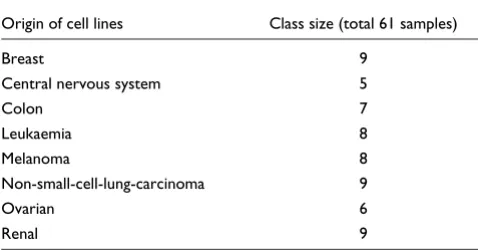
In the NCI 60 data [12], cDNA microarrays were used to study the expression of approximately 60 cell lines derived from tumors with different sites of origin (see Table 1). We used the same pre-processed dataset as in Dudoit et al. [23], which consists of log expression ratios of 5,244 genes over 61 exper-iments. Two prostate and one unknown cell lines from the original data [12] were excluded in their analysis because of their small class sizes. Only one leukemia and one breast can-cer cell line were repeated three times, and hence there are no repeated measurements or variability estimates available for all 61 samples. These repeated experiments of the leukemia and breast cancer cell lines are treated as individual samples. In addition, no additional test set is available for this data. To compare our results with those of Dudoit et al. [23], we adopted their 2:1 scheme in which one third of the samples are reserved as a test set.
Specifically, we randomly divided each class in the original data (61 experiments) into roughly three parts such that the training set consists of a total of 43 experiments and the test set consists of a total of 18 experiments. Table 2 gives the class sizes of the training and test sets. The optimal parameters are determined using cross-validation on the training set with 43 samples, and these optimal parameters are used to classify the 18 samples in the test set. We repeated this random parti-tion of the original data into three parts multiple times.
Multiple tumor data
The multiple tumor dataset [10] consists of a large number of tumor samples spanning 14 different tumor types hybridized to Affymetrix chips. On the Affymetrix platform, each target gene is represented by 11-20 short oligo probes of approxi-mately 25 base-pairs (bp). Our goal is to take advantage of the variability over different oligos for the same genes using our EWUSC algorithm. We pre-processed the raw multiple tumor data with the log scale robust multi-array analysis (RMA) measure [27] implemented in the BioConductor project. The RMA measure is a summary statistic for the expression levels over all the different oligos for the same gene. The standard error of the RMA measure is a variability estimate of the expression level over the different oligos representing the same target gene. In order to obtain the RMA measures and their associated standard errors on the multiple tumor data, the raw data (.cel files) are necessary. Because we have access to only a subset of the raw multiple tumor data, we used a sub-set of the original data in our study. The subsub-set of multiple tumor data we used consists of 7,129 genes, 96 samples in the training set, and 27 samples in the test set. These samples span 11 different tumor types (Table 3). The smallest class size is four on the training set, and hence, four-fold cross-valida-tion (m = 4) is used on this data.
Breast cancer data
[image:5.612.54.293.120.245.2]The breast cancer data [14] consists of primary breast tumor samples hybridized to cDNA arrays containing approximately 25,000 genes. Two hybridizations were carried out for each sample using a dye-reversal technique. Hence, there are four repeated measurements for each gene and each sample. The values of log expression ratios are also available. These p-values are results of the four repeated measurements and an error model based on extensive control experiments [29]. A p-value close to 1 represents low confidence that an expression ratio is significantly different from 1, while a Table 1
Tumor types and class sizes of the NCI 60 dataset
Origin of cell lines Class size (total 61 samples)
Breast 9
Central nervous system 5
Colon 7
Leukaemia 8
Melanoma 8
Non-small-cell-lung-carcinoma 9
Ovarian 6
Renal 9
Tumor types and class sizes of the original full data with a total of 61 experiments.
Table 2
Tumor types and class sizes of the randomly partitioned training and test sets of the NCI 60 dataset
Origin of cell lines Training set
(total 43)
Test set (total 18)
Breast 6 3
Central nervous system 4 1
Colon 5 2
Leukaemia 6 2
Melanoma 6 2
Non-small-cell-lung-carcinoma 6 3
Ovarian 4 2
Renal 6 3
[image:5.612.311.554.564.700.2]p-value close to 0 represents high confidence that an expres-sion ratio is significantly different from 1. We converted these p-values into error estimates of log ratios, which are used in our EWUSC algorithm.
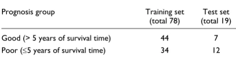
The breast cancer dataset consists of approximately 25,000 genes, 78 samples in the training set, and 19 samples in the test set. van't Veer et al. [14] divided these samples into the good and poor prognosis groups, which have greater than 5 and less than 5 years of survival time respectively. Hence, there are two classes in this dataset (see Table 4). We per-formed 10-fold cross-validation (m = 10) on the breast cancer data.
Synthetic data
We also created synthetic datasets to compare the perform-ance of our algorithms. Our approach is to start with 'pat-terned genes' which have a different expression pattern in each class, and are therefore relevant in classifying unknown samples. The next step is to introduce noise (variation in both the class and non-class values) to these patterned genes in order to reflect 'real-life' data. Finally, 'non-patterned genes', which are irrelevant in classifying samples, are added to these synthetic datasets. Even with this simple synthetic
data-generation approach, generating sensible synthetic data turned out to be a nontrivial task. There are two parameters that control the noise levels in the synthetic datasets, the bio-logical noise level (α) and the technical noise level (λ). The biological noise level (α) controls the level of biological noise within each class (and hence, the signal-to-noise ratio) such that the classes are less separable with a higher α. The techni-cal noise level (λ) controls the noise level over repeated meas-urements such that a high λ indicates relatively noisy repeated measurements. The primary difficulty in generating synthetic data is setting the parameters of α and λ, and the proportion of the patterned genes. As it is not obvious how to set these parameters to reflect 'real-life' data, we experi-mented with different parameter settings, such as different biological noise levels: low (α = 0.1 with signal-to-noise ratio approximately 20), medium (α = 1 with signal-to-noise ratio approximately 2), or high (α = 2 with signal-to-noise ratio approximately 1); and low (λ = 1) or high (λ = 5 or 10) techni-cal noise. We also experimented with different proportions of patterned genes, and concluded that this parameter does not have any significant impact on the results.
Another issue in generating 'realistic' synthetic data involves the generation of non-patterned genes that are irrelevant in distinguishing the classes. We addressed this issue by random sampling with replacement from a real dataset (that is, the breast cancer dataset [14]). Specifically, for each non-pat-terned gene, we randomly sample a gene g from the breast cancer data, and then randomly sample from the experiments of gene g in the breast cancer data such that these non-pat-terned genes would not show any class-specific expression patterns but would show realistic variations in expression lev-els over all classes.
In particular, our synthetic training sets consist of 1,000 genes, 80 samples, and 4 classes such that there are 20 sam-ples in each class. Our synthetic test sets consist of 1,000 genes and 40 samples with 10 samples in each class. We gen-erated 64 patterned genes which have a different expression pattern in each class, for example, genes that are upregulated (or downregulated) in only m of the four classes, where m = 1, 2, 3. In addition, there are five duplicates of each of these 64 patterned genes such that there are a total of 320 patterned genes and (1,000 - 320 = 680) non-patterned genes. Ideally, the perfect classification algorithm would select only one of these five copies of the patterned genes. We also investigated the effect of the number of repeated measurements by gener-ating synthetic datasets with 1, 4 or 20 repeated measure-ments. These synthetic datasets are available from our supplementary website [30].
Assessment criteria
Prediction accuracy [image:6.612.55.298.130.297.2]As the class information for the test sets is available, we define prediction accuracy as the percentage of correct Table 3
Tumor types and class sizes for the training set and test set of the subset of multiple tumor data used in this study
Tumor type Training set (total 96) Test set (total 27)
Breast 7 0
Lung 4 2
Colorectal 7 3
Lymphoma 14 5
Melanoma 5 0
Uterus 7 2
Leukemia 23 6
Renal 5 3
Pancreas 7 0
Mesotheolima 8 3
CNS 9 3
Table 4
Prognosis groups and class sizes of the training set and test set of the breast cancer data
Prognosis group Training set
(total 78)
Test set (total 19)
Good (> 5 years of survival time) 44 7
[image:6.612.56.296.377.439.2]comm
en
t
re
v
ie
w
s
re
ports
refer
e
e
d
re
sear
ch
de
p
o
si
te
d r
e
se
a
rch
interacti
o
ns
inf
o
rmation
classifications on the test set. The class information on a test set is used only to evaluate the performance of classification and feature-selection algorithms, and is unknown to the algo-rithms.
Number of relevant features
One of the goals of classification is to select a minimal set of relevant genes (or features) that can be used in future diagno-sis or classification of tissue samples. We judge each method by the total number of relevant features required for optimal classification accuracy. A small set of relevant genes is desir-able because it is more cost-effective in the development of diagnostic tools based on the results of expression analysis. For example, the cost of an RT-PCR test to classify patient samples is directly proportional to the number of genes which must be tested to make the diagnosis. As shown below, both the USC and EWUSC methods usually result in a significant reduction in the numbers of selected genes for classification. We feel this represents a major advance in classification algorithms.
Feature stability
Because relevant genes are derived from the training set and the choice of the training set is often arbitrary, a set of rele-vant genes that is insensitive to the training sets used would be desirable. Hence, we define feature stability as the level of agreement between the set of relevant genes chosen in each fold of the cross-validation data with the set of relevant genes chosen using the full training set. Specifically, for each fold of the cross-validation data and for each set of parameters (∆ and ρ0), we compute the Jaccard index [31] which measures the level of agreement between the set of relevant genes cho-sen in this fold and the set chocho-sen using the full training set. The Jaccard index lies between 0 and 1. A high Jaccard index (close to 1) implies high level of agreement, and hence, high feature stability (a mathematical definition of the Jaccard index can be found in the section Details of algorithms, below). We define feature stability of one cross-validation run for a given set of parameters (∆ and ρ0) as the average Jaccard index over all m folds of cross-validation. In our experiments, we usually have five random runs of cross-validation; hence we adopt the average Jaccard index over these five random runs of cross-validation as our measure of overall feature sta-bility for given parameters (∆ and ρ0).
Results on the NCI 60 data
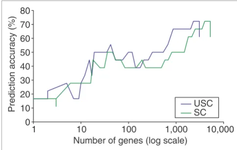
As variability estimates are not available on the NCI 60 data, we compared the prediction accuracy from USC and SC (Fig-ure 1; and Fig(Fig-ure S14 of [30]). We showed that USC generally produces higher prediction accuracy than SC using the same number of relevant genes (Figure 1). In particular, USC requires 44% of the available genes (2,315 out of 5,244 genes) to achieve a prediction accuracy of 72%, whereas SC requires 77% of genes (3,998 out of 5,244 genes) to achieve the same prediction accuracy. Our results show that the removal of
highly correlated genes reduces the number of selected fea-tures while achieving comparable error rates.
Like Dudoit et al. [23] we observed high error rates on this dataset (around 40-60% using 10-200 relevant genes). USC produces comparable error rates to the results reported in Dudoit et al. [23] using roughly the same number of relevant genes. However, our USC algorithm allows the optimal parameters (which indirectly control the number of selected genes) to be determined. In this case, the optimal parameters produce an error rate of approximately 28% on the cross-val-idation data. We repeated the random partition of the full dataset with 61 samples into a training set with 43 samples and a test set with 18 samples multiple times, and obtained similar results on different random partitions of the original dataset.
Results on the multiple tumor data
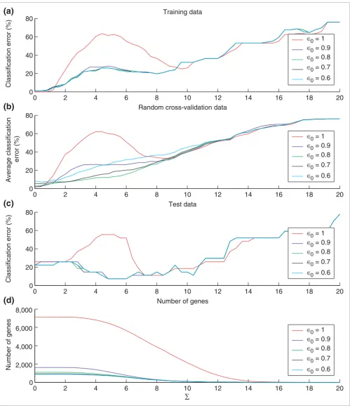
[image:7.612.312.554.87.240.2]Figure 2 shows the results of applying EWUSC to the training set, four-fold cross-validation data, and test set of the multi-ple tumor data over a range of shrinkage thresholds (∆) and correlation thresholds (ρ0). In Figure 2a,c the percentage of classification errors is plotted against ∆ on the training and test sets respectively. In Figure 2b, the average percentage of errors is plotted against ∆ over five random runs of cross-val-idation. The optimal parameters (∆ and ρ0) are determined from the cross-validation results. Figure 2a-c shows that pre-diction accuracy is increased (lower percentage of errors) when ρ0 < 1 over most values of ∆ (especially 2 ≤∆≤ 7) on the training set, cross-validation data and test set. This shows that removing highly correlated genes increases prediction Comparison of prediction accuracy of USC and SC on the NCI 60 data Figure 1
Comparison of prediction accuracy of USC and SC on the NCI 60 data. The percentage of prediction accuracy is plotted against the number of relevant genes using the USC algorithm at ρ0 = 0.6 and the SC algorithm
(USC at ρ0 = 1.0). The horizontal axis is shown on a log scale. Because no
independent test set is available for this data, we randomly divided the samples in each class into roughly three parts multiple times, such that a third of the samples are reserved as a test set. Thus the training set consists of 43 samples and the test set of 18 samples. The graph represents typical results over these multiple random runs.
100 10
1 1,000 10,000
Number of genes (log scale)
Prediction accuracy (%) USCSC
Prediction accuracy on the multiple tumor data using the EWUSC algorithm over the range of ∆ from 0 to 20 Figure 2
Prediction accuracy on the multiple tumor data using the EWUSC algorithm over the range of ∆ from 0 to 20. The percentage of classification errors is plotted against ∆ on (a) the full training set (96 samples) and (c) the test set (27 samples). In (b) the average percentage of errors is plotted against ∆ on the cross-validation data over five random runs of fourfold cross-validation. In (d), the number of relevant genes is plotted against ∆. Different colors are used to specify different correlation thresholds (ρ0 = 0.6, 0.7, 0.8, 0.9 or 1). Results of ρ0 < 0.6 are shown in Figure S1 on [30]. Optimal parameters are
inferred from the cross-validation data in (b).
0 2 4 6 8 10 12 14 16 18 20
0 20 40 60 80
Classification error (%)
Classification error (%)
0 2 4 6 8 10 12 14 16 18 20
0 20 40 60 80
Average classification
error (%)
0 2 4 6 8 10 12 14 16 18 20
0 20 40 60 80
0 2 4 6 8 10 12 14 16 18 20
0
∆
Number of genes
ρ0 = 1
ρ0 = 0.9
ρ0 = 0.8
ρ0 = 0.7
ρ0 = 0.6
Training data
Random cross-validation data
Test data
Number of genes
2,000 4,000 6,000 8,000
ρ0 = 1
ρ0 = 0.9
ρ0 = 0.8
ρ0 = 0.7
ρ0 = 0.6
ρ0 = 1
ρ0 = 0.9
ρ0 = 0.8
ρ0 = 0.7
ρ0 = 0.6
ρ0 = 1
ρ0 = 0.9
ρ0 = 0.8
ρ0 = 0.7
ρ0 = 0.6
(a)
(b)
(c)
comm
en
t
re
v
ie
w
s
re
ports
refer
e
e
d
re
sear
ch
de
p
o
si
te
d r
e
se
a
rch
interacti
o
ns
inf
o
rmation
accuracy. In addition, Figure 2d shows that the number of rel-evant genes is drastically reduced when genes with correla-tion threshold (ρ0) above 0.9 are removed. From Figure 2b, the average cross-validation error rate gradually reduces when the correlation threshold ρ0 is decreased from 1 to 0.9 to 0.8, but the average error rate increases when ρ0 < 0.8. (This observation also holds for ρ0 < 0.6, which are not shown in Figure 2 for clarity.) Therefore, the optimal ρ0 is estimated to be 0.8.
EWUSC produces the minimum average number of cross-val-idation errors at ∆ = 0 and ρ0 = 0.9 using 1,626 relevant genes, which achieves 78% prediction accuracy. However, ∆ = 0 is an unsatisfactory shrinkage threshold because we would prefer relevant genes to have class centroids significantly different from their overall centroids. Moreover, the average error rate starts to increase almost linearly when ∆ is greater than 6 on the cross-validation data. This 'bend' is more obvious Figure S1(e) on [30], which shows the error rate for each of the five random runs of fourfold cross-validation for ∆ = 0 to 14. The optimal ∆ is estimated to be 5.6. When ∆ = 5.6 and ρ0 = 0.8, the prediction accuracy is 93% and the number of relevant genes is 680 (out of a total of 7,129 genes).
We also applied the USC and SC algorithms to the multiple tumor data and obtained similar results, except that the error rates are generally higher. Similarly, USC produces the mini-mum average number of cross-validation errors at ∆ = 0 and ρ0 = 0.9 using 1634 relevant genes, which achieves 74% pre-diction accuracy. SC produces the minimum average number of cross-validation errors at ∆ = 0.4 using all 7,129 genes. On the other hand, the optimal parameters (∆, ρ0) can be esti-mated by visual observation of 'bends' in the cross-validation curves. In particular, when ∆ = 5.6 and ρ0 = 0.8, the predic-tion accuracy is 85% and the number of relevant genes is 735 using the USC algorithm (see Figure S2 on [30] for detailed results).
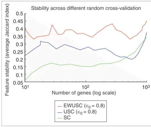
We also compared feature stability of the EWUSC and USC algorithms at correlation threshold (ρ0) = 0.8 with the SC algorithm [17] (which is equivalent to USC at ρ0 = 1) over dif-ferent numbers of relevant genes (Figure 3), and showed that EWUSC produces higher feature stability (higher average Jaccard index) than the USC and SC algorithms. The rela-tively high feature stability is due to relarela-tively high numbers of common features selected in different runs of cross-valida-tion (see Figure S5 on [30]). We also showed that EWUSC almost always selects relatively more stable sets of relevant genes than USC (even over other correlation thresholds that are not shown). Hence, our results demonstrate that incorpo-rating variability estimates over repeated measurements yields higher feature stability.
Comparison with published results
Ramaswamy et al. [10] reported 78% classification accuracy on the multiple tumor data using SVMs combined using the
one-versus-all approach. In contrast, our EWUSC algorithm achieves a classification accuracy of 93% on the test set of the multiple tumor data. As we used a subset of the original multiple tumor data and pre-processed the raw data using the RMA measures [27], we evaluated the performance of SVM combined with the one-versus-all method on the identical pre-processed subset of multiple tumor data used in our experiments with the EWUSC and the USC algorithms. In our comparison study, we used the signal to noise (S2N) measures [9] to select relevant features for each binary SVM classifier. To produce directly comparable results, we used the exact same five splits of the training set into cross-valida-tion data.
Figure 4 compares the prediction accuracy on the test set of the multiple tumor data using the EWUSC and USC algo-rithms at the estimated optimal correlation threshold (ρ0 = 0.8), the SC algorithm [17] and SVM (with S2N for feature selection). There are a few observations from Figure 4. First, USC produces higher prediction accuracy than SC using the same number of relevant genes. As SC is equivalent to USC at ρ0 = 1, our results show that removing highly correlated genes reduces the number of relevant genes and improves predic-tion accuracy. Second, EWUSC generally produces higher prediction accuracy than USC using the same number of rel-evant genes, except when both the number of relrel-evant genes and prediction accuracy is low. This shows that we can poten-tially improve prediction accuracy by taking advantage of error estimates in the data.
[image:9.612.311.554.86.290.2]Comparison of feature stability of EWUSC, USC and SC on the multiple tumor data
Figure 3
Comparison of feature stability of EWUSC, USC and SC on the multiple tumor data. The average Jaccard index is plotted against the number of relevant genes over five random runs of fourfold cross-validation using EWUSC and USC at ρ0 = 0.8 and SC. A high average Jaccard index
indicates high feature stability. The EWUSC algorithm selects the most stable features. Note that the horizontal axis is shown on a log scale.
Feature stability (average Jaccard index) Number of genes (log scale)
Stability across different random cross-validation
EWUSC (ρ0 = 0.8) USC (ρ0 = 0.8) SC
0.5
0.45 0.4
0.35 0.3
0.25 0.2
0.15 0.1
0.05
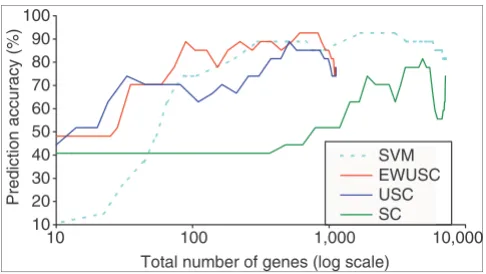
Third, our SVM results (on a subset of the multiple tumor data pre-processed with RMA measures) are generally much better than the published result of 78% [10] (on the full dataset pre-processed with MAS 4). Fourth, SVM with S2N as our feature-selection method produces high prediction accu-racy at the expense of using a lot of relevant genes. For exam-ple, SVM requires a total of 1,699 genes over all the binary classifiers to achieve 93% prediction accuracy, whereas our EWUSC algorithm requires only 610 relevant genes to achieve the same prediction accuracy. If we are willing to trade off prediction accuracy with the number of relevant genes, EWUSC achieves 89% prediction accuracy with only 89 relevant genes.
Results on the breast cancer data
We applied the EWUSC, USC and SC algorithms to the breast cancer data, and compared the prediction accuracy of the three algorithms at their optimal correlation thresholds (ρ0 = 0.7 or 0.6), and the SC algorithm (USC at ρ0 = 1). The results are shown in Figure 5. In general, EWUSC produces higher prediction accuracy than USC and SC when the number of relevant genes is less than 1,000 (which is the range of interest). In particular, EWUSC produces fewer classification errors on the test set at its optimal parameters (two errors at ∆ = 0.8 and ρ0 = 0.7) than USC at its optimal parameters (four errors at ∆ = 1.15 and ρ0 = 0.6).
Moreover, EWUSC generally selects relevant genes with rela-tively small error bars (or low p-values). For example, there are two genes with p-values equal to 1 across all 78 samples in the training set. In other words, we have very low confidence that the expression ratios of these two genes are changed in
any of the 78 samples of the training set. It is undesirable to classify new samples using these genes that do not show any expression patterns. With EWUSC (which takes error esti-mates into consideration), these two genes are eliminated for all ∆ > 0. On the contrary, one of these two genes is selected as a relevant gene by USC for ∆ = 0, 0.05, ..., 0.7 at ρ0 = 1.
The detailed results of applying the EWUSC and USC algo-rithms to the breast cancer data are shown in Figures S8 and S9 on [30]. Surprisingly, removing highly correlated genes does not produce any considerable improvement in predic-tion accuracy and does not drastically reduce the number of relevant genes. This is probably due to the fact that the numbers of classification errors on the cross-validation data are not well correlated with those on the test set (see [30]). Because the test set is an additional independent dataset, there might be some heterogeneity between the training and test sets. Nevertheless, USC achieves comparable prediction accuracy to SC using relatively fewer selected genes (under 100 genes) over different correlation thresholds ρ0.
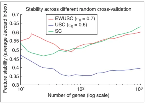
We compared the feature stability of EWUSC, USC and SC at their optimal correlation thresholds ρ0 in Figure 6. We showed that EWUSC and SC produce relatively stable rele-vant features than USC. The detailed comparison of feature stability in terms of the average numbers of true/false posi-tives/negatives are shown in Figures S12 and S13 on [30]. The relatively high feature stability of SC is due to its relatively high true-positive rate (common genes chosen in both ran-dom cross-validation and using the entire training set), and its relatively low false-negative rate (genes chosen using the entire training set but not in the cross-validation data). How-ever Figure S12 in [30] shows that this effect is drastic at high numbers of relevant genes and is relatively less significant at Comparison of prediction accuracy of EWUSC, USC, SVM and SC
[image:10.612.57.300.85.222.2]algorithms on the multiple tumor data Figure 4
Comparison of prediction accuracy of EWUSC, USC, SVM and SC algorithms on the multiple tumor data. The horizontal axis shows the total number of distinct genes selected over all binary SVM classifiers on a log scale. Some results are not available on the full range of the total number of genes. For example, the maximum numbers of selected genes for EWUSC and USC are roughly 1,000. The reported prediction accuracy is 78% [10] using all 16,000 available genes on the full data. The EWUSC algorithm achieves 89% prediction accuracy with only 89 genes. With 680 genes, EWUSC produces 93% prediction accuracy.
10 100 1,000 10,000
Total number of genes (log scale)
Prediction accuracy (%)
SVM EWUSC USC SC 10
20 30 40 50 60 70 80 90 100
[image:10.612.315.556.87.246.2]Comparison of prediction accuracy of EWUSC, USC and SC on the breast cancer data
Figure 5
Comparison of prediction accuracy of EWUSC, USC and SC on the breast cancer data. The percentage of prediction accuracy is plotted against the number of relevant genes using the EWUSC algorithm at ρ0 = 0.7, the USC algorithm at ρ0 = 0.6 and the SC algorithm (USC at ρ0 = 1.0). Note that the horizontal axis is shown on a log scale.
Total number of genes (log scale)
Prediction accuracy (%)
Test data
EWUSC (ρ0 = 0.7)
USC (ρ0 = 0.6)
SC
60
101 102 103 104
comm
en
t
re
v
ie
w
s
re
ports
refer
e
e
d
re
sear
ch
de
p
o
si
te
d r
e
se
a
rch
interacti
o
ns
inf
o
rmation
our optimal parameters with approximately 100 to 300 rele-vant genes.
Results on the synthetic data
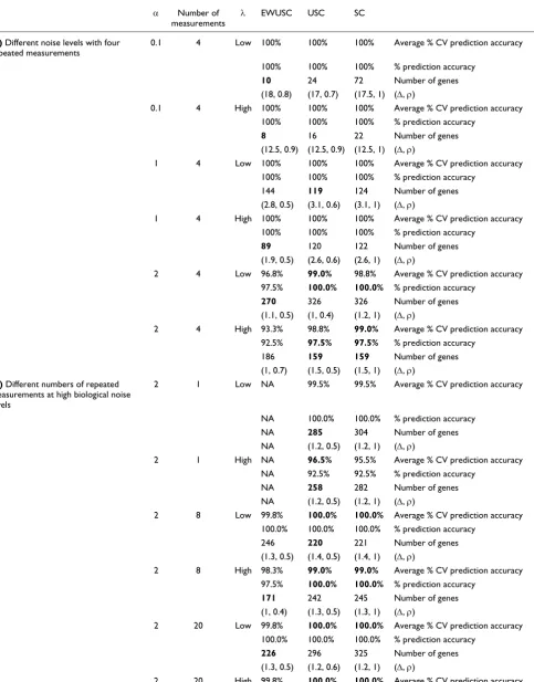
We compared the performance of EWUSC, USC and SC on synthetic datasets with different numbers of repeated measurements, different biological and technical noise levels. As the biological noise levels of typical real microarray data-sets are not known, we generated synthetic datadata-sets with four repeated measurements at different biological noise levels (α = 0.1, 1 or 2) and some typical results are shown in Table 5a. Our complete results are shown in Tables S1, S2 and S3 on [30]. In most cases, USC achieves better or comparable pre-diction accuracy (lower number of errors on the test set) than SC using fewer relevant genes. There are a few exceptions to this observation (see [30]). The optimal parameters (∆, ρ0) are determined from the minimum average number of cross-validation errors. In some cases, there are very small differ-ences between the average numbers of cross-validation errors of two sets of parameters, and the set of parameters that pro-duces a slightly higher average cross-validation error rate yields fewer relevant genes. Therefore, this 'exception' is due to the fact that the optimal parameters are not derived from the random cross-validation data. At low biological noise level (α), the inference of optimal parameters is obvious and USC always yields fewer relevant genes than SC (see Table S2 on [30]). This observation demonstrates the power of remov-ing highly correlated genes in the USC algorithm. Our results also showed that EWUSC consistently achieves the same pre-diction accuracy using fewer relevant genes at low biological noise (α = 0.1, with signal-to-noise ratio approximately 20) at different technical noise levels (Table 5a). However, as α is
increased, the performance of EWUSC compared to USC deteriorates. For example, EWUSC selects more relevant genes than USC at low technical noise level but it selects fewer relevant genes than USC at α = 1 (with signal-to-noise ratio approximately 2). The relative performance of EWUSC is even less favorable at high biological noise level (α = 2 with signal-to-noise ratio roughly 1). The results in Table 5a sug-gest that EWUSC is the method of choice when the classes are relatively separable (at low biological noise and high signal-to-noise ratio), but USC would be the method of choice at high biological noise.
In general, the performance of EWUSC increases as the number of repeated measurements increases. In particular, we studied the effect of the number of repeated measurements on the relative performance of EWUSC, USC and SC at high biological noise (α = 2). The prediction accuracy results using 1, 8 or 20 repeated measurements at high biological noise (α = 2) are shown in Table 5b. The results at α = 2 with four repeated measurements are shown in Table 5a. USC typically outperforms SC by selecting fewer relevant genes over different numbers of repeated measure-ments. In addition, we showed that EWUSC usually selects fewer relevant genes than USC at high biological noise when there are 20 repeated measurements. However, when the bio-logical noise level is high (with signal-to-noise ratio approxi-mately 1) and the number of repeated measurements is low (1, 4 or 8), USC usually selects fewer relevant genes than EWUSC.
Table 5a,b shows that EWUSC produces lower prediction accuracy than USC at high biological noise when there are few repeated measurements. However, the levels of biological noise on real microarray datasets are not known. In practice, we recommend users of our algorithms to compare the average numbers of errors on the cross-validation data and the numbers of relevant genes from the EWUSC and USC algorithms, and then select the algorithm that produces lower average cross-validation errors using fewer relevant genes. In most cases, the prediction accuracy on the test set shows the same trend as the average number of cross-validation errors.
It is interesting that prediction accuracy is not necessarily reduced and the number of relevant genes is not necessarily increased at higher technical noise levels. However, predic-tion accuracy is generally reduced and the number of relevant genes is typically increased at higher biological noise levels (see Additional data files Tables S1, S2 and S3 at [30]). All three algorithms (EWUSC, USC and SC) produce comparable feature stability at different noise levels when the number of relevant genes is below 300 (see Figures S20, S21 at [30]).
Summary of results on real data
Table 6 summarizes our prediction accuracy results using the EWUSC, USC and SC algorithms on the NCI 60 data, multiple Comparison of feature stability of EWUSC, USC and SC on the breast
[image:11.612.54.297.85.257.2]cancer data Figure 6
Comparison of feature stability of EWUSC, USC and SC on the breast cancer data. The average Jaccard index is plotted against the number of relevant genes over five random runs of 10-fold cross-validation using the EWUSC algorithm at ρ0 = 0.7, the USC algorithm at ρ0 = 0.6 and the SC algorithm (USC at ρ0 = 1). The EWUSC algorithm produces relatively
more stable features when the number of relevant genes is small.
Feature stability (average Jaccard index)
Number of genes (log scale)
Stability across different random cross-validation
EWUSC (ρ0 = 0.7)
USC (ρ0 = 0.6)
SC 0.65
0.7
0.6
0.55
0.5
0.45
0.4
0.35
0.3
Table 5
Comparison of classification accuracy results from EWUSC, USC and SC on synthetic datasets at optimal parameters
α Number of
measurements
λ EWUSC USC SC
(a) Different noise levels with four repeated measurements
0.1 4 Low 100% 100% 100% Average % CV prediction accuracy
100% 100% 100% % prediction accuracy
10 24 72 Number of genes
(18, 0.8) (17, 0.7) (17.5, 1) (∆, ρ)
0.1 4 High 100% 100% 100% Average % CV prediction accuracy
100% 100% 100% % prediction accuracy
8 16 22 Number of genes
(12.5, 0.9) (12.5, 0.9) (12.5, 1) (∆, ρ)
1 4 Low 100% 100% 100% Average % CV prediction accuracy
100% 100% 100% % prediction accuracy
144 119 124 Number of genes
(2.8, 0.5) (3.1, 0.6) (3.1, 1) (∆, ρ)
1 4 High 100% 100% 100% Average % CV prediction accuracy
100% 100% 100% % prediction accuracy
89 120 122 Number of genes
(1.9, 0.5) (2.6, 0.6) (2.6, 1) (∆, ρ)
2 4 Low 96.8% 99.0% 98.8% Average % CV prediction accuracy
97.5% 100.0% 100.0% % prediction accuracy
270 326 326 Number of genes
(1.1, 0.5) (1, 0.4) (1.2, 1) (∆, ρ)
2 4 High 93.3% 98.8% 99.0% Average % CV prediction accuracy
92.5% 97.5% 97.5% % prediction accuracy
186 159 159 Number of genes
(1, 0.7) (1.5, 0.5) (1.5, 1) (∆, ρ)
(b) Different numbers of repeated measurements at high biological noise levels
2 1 Low NA 99.5% 99.5% Average % CV prediction accuracy
NA 100.0% 100.0% % prediction accuracy
NA 285 304 Number of genes
NA (1.2, 0.5) (1.2, 1) (∆, ρ)
2 1 High NA 96.5% 95.5% Average % CV prediction accuracy
NA 92.5% 92.5% % prediction accuracy
NA 258 282 Number of genes
NA (1.2, 0.5) (1.2, 1) (∆, ρ)
2 8 Low 99.8% 100.0% 100.0% Average % CV prediction accuracy
100.0% 100.0% 100.0% % prediction accuracy
246 220 221 Number of genes
(1.3, 0.5) (1.4, 0.5) (1.4, 1) (∆, ρ)
2 8 High 98.3% 99.0% 99.0% Average % CV prediction accuracy
97.5% 100.0% 100.0% % prediction accuracy
171 242 245 Number of genes
(1, 0.4) (1.3, 0.5) (1.3, 1) (∆, ρ)
2 20 Low 99.8% 100.0% 100.0% Average % CV prediction accuracy
100.0% 100.0% 100.0% % prediction accuracy
226 296 325 Number of genes
(1.3, 0.5) (1.2, 0.6) (1.2, 1) (∆, ρ)
comm
en
t
re
v
ie
w
s
re
ports
refer
e
e
d
re
sear
ch
de
p
o
si
te
d r
e
se
a
rch
interacti
o
ns
inf
o
rmation
tumor data and breast cancer data at optimal parameters. In general, we showed that using variability over repeated meas-urements to down-weight noisy genes/experiments and the removal of highly correlated genes usually reduce the number of relevant genes necessary for accurate class predictions. In addition, using variability of repeated measurements to down-weight noisy genes/experiments generally increases feature stability. Hence, our EWUSC and USC algorithms represent advances over the published SC algorithm [17].
On the NCI 60 data, USC generally produces higher predic-tion accuracy than SC using the same number of relevant genes. This result shows that the removal of highly correlated genes reduces the number of genes necessary for class prediction while achieving comparable or higher prediction accuracy.
On the multiple tumor data, EWUSC has the following advan-tages over other methods: EWUSC produces higher predic-tion accuracy and selects fewer relevant genes than all other approaches. In particular, EWUSC achieves 93% of predic-tion accuracy using less than 10% of the genes compared to 78% of prediction accuracy using all the available genes in the published results [10]. Each of the binary SVM classifiers chooses a different subset of relevant genes while our EWUSC algorithm uses only one set of relevant genes for all classes.
van't Veer et al. [14] reported two classification errors using 70 relevant genes on the test set of the breast cancer data (out of a total of 19 samples). Our EWUSC produces the same number of errors on the test set with 271 relevant genes. How-ever, our EWUSC algorithm has the following advantages over the prognostic classifier used in [14]. No ad hoc filtering step is necessary. The EWUSC algorithm automatically
avoids choosing noisy genes. The EWUSC algorithm can be applied to data with any number of classes. This is in contrast to the prognostic classifier, which is not applicable to the mul-tiple tumor data (which consists of 11 classes) or the NCI 60 data (which consists of 8 classes).
Comparison of USC, EWUSC and SC
algorithms
The key characteristics of EWUSC, USC and SC are summa-rized in Table 7. We illustrated the EWUSC and USC algo-rithm on both real and synthetic datasets. Our results on real data are summarized in Table 6. We compared the performance of USC with SC, and showed that USC typically achieves comparable prediction accuracy using a smaller set of relevant genes on both real and synthetic datasets. We showed that the step of removing highly correlated genes in USC is effective in reducing the number of relevant genes without sacrificing prediction accuracy, and hence, USC is an improvement over SC.
We also compared the performance of EWUSC (which down-weights noisy genes and noisy experiments) with USC on both real and synthetic datasets. On real microarray datasets (mul-tiple tumor data and breast cancer data), we showed that EWUSC usually achieves higher or comparable feature stability using a smaller set of relevant genes, and EWUSC avoids choosing noisy relevant genes for classification of sam-ples. Hence, we showed that using variability over repeated measurements improves classification and feature-selection results. Moreover, we compared EWUSC with other existing classification and feature-selection algorithms, and showed that EWUSC produces better or at least comparable results than previously reported results on real datasets (see Table
100.0% 100.0% 100.0% % prediction accuracy
221 252 252 Number of genes
(0.9, 0.6) (1.3, 0.5) (1.3, 1) (∆, ρ)
Synthetic datasets were generated at different levels of biological noise (α) and technical noise (λ). The average percentage of cross validation (% CV) accuracy, the percentage of prediction accuracy on the test set, the number of relevant genes at the optimal parameters (∆, ρ0) are shown. For each synthetic dataset, the algorithm with the maximum percentage of average cross validation accuracy, maximum prediction accuracy, or the minimum number of relevant genes is shown in bold. (a) Typical classification accuracy results using synthetic datasets with four repeated measurements at different biological noise levels (α = 0.1, 1 or 2) and difference technical noise levels (λ = 1, 5 or 10). When the biological noise level is low (α = 0.1), EWUSC consistently achieves the same prediction accuracy using fewer relevant genes at various technical noise levels. However, at medium biological noise level (α = 1), EWUSC typically outperforms USC and SC at high technical noise level and not at low technical noise level. When the biological noise level is high (α = 2), EWUSC is often not the method of choice. (b) Typical classification accuracy results using synthetic datasets at high biological noise level (α = 2) with 1, 8, or 20 repeated measurements at different technical noise levels. When there is no repeated
[image:13.612.68.547.119.162.2]measurement (the number of repeated measurements = 1), there are no variability estimates over repeated measurements and hence, EWUSC is reduced to USC. The results with four repeated measurement at α = 2 are shown in (a). Our results over multiple synthetic datasets showed that EWUSC only outperforms USC with a large number of repeated measurements (20) at high biological noise (α = 2). We also showed that USC typically outperforms SC by choosing a smaller number of relevant genes in most scenarios (over different biological and technical noise levels, and different numbers of repeated measurements).
Table 5 (Continued)
6). On the other hand, our results on synthetic datasets showed that EWUSC is usually the method of choice when the classes are well separated (that is, when biological noise is low or signal-to-noise ratio is high).
Our main contribution is that we use cross-validation to select a correlation threshold (ρ0) for the removal of highly corre-lated genes. This idea is adopted in both USC and EWUSC, which in turn take advantage of the interdependence of genes without sacrificing prediction accuracy. Our second major contribution is that we adopted the error-weighted method in our integrated feature-selection and classification algorithm, EWUSC. To the best of our knowledge, EWUSC is the only classification algorithm applicable to microarray data with any number of classes that takes advantage of variability in repeated measurements.
There are many directions for future work. The error-weighted idea can be applied to other distance-based classifi-cation algorithms, for example, the k-nearest neighbour, which was shown to achieve high prediction accuracy [23].
Our next step is to compare the performance of the EWUSC and USC algorithms with a wide range of other classification and feature selection algorithms. One problem in the litera-ture is that researchers often use different pre-processed sub-sets of published array data, which makes direct comparisons of published results difficult. Therefore, there is a need to conduct a large-scale evaluation study of various classifica-tion and feature selecclassifica-tion algorithms on microarray data.
Details of algorithms
The SC algorithm of Tibshirani et al. [17]
Let xij be the expression level for gene i = 1, 2, ..., p and sam-ples j = 1, 2, ..., n. Suppose there are a total of K classes, and let Ck be the set of all nk samples in class k. The overall cen-troid of gene i is,
,
[image:14.612.57.545.116.345.2]and the class centroid of class k and gene i is, Table 6
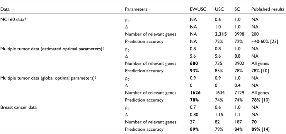
Summary of prediction accuracy results
Data Parameters EWUSC USC SC Published results
NCI 60 data* ρ0 NA 0.6 1.0 NA
∆ NA 1.0 1.0 NA
Number of relevant genes NA 2,315 3998 200
Prediction accuracy NA 72% 72% ~40-60% [23]
Multiple tumor data (estimated optimal parameters)† ρ
0 0.8 0.8 1.0 NA
∆ 5.6 5.6 8.8 NA
Number of relevant genes 680 735 3902 All genes
Prediction accuracy 93% 85% 78% 78% [10]
Multiple tumor data (global optimal parameters)‡ ρ
0 0.9 0.9 1.0 NA
∆ 0 0 0.4 NA
Number of relevant genes 1626 1634 7129 All genes
Prediction accuracy 78% 74% 74% 78% [10]
Breast cancer data ρ0 0.7 0.6 1.0 NA
∆ 0.80 1.15 1.1 NA
Number of relevant genes 271 82 187 70
Prediction accuracy 89% 79% 84% 89% [14]
The optimal parameters (ρ0 and ∆), number of relevant genes chosen, and prediction accuracy for the NCI 60 data, multiple tumor data and breast cancer data are summarized here. Both EWUSC (error-weighted, uncorrelated shrunken centroid) and USC (uncorrelated shrunken centroid) were motivated by SC (shrunken centroid) [17]. Both EWUSC and USC take advantage of interdependence between genes by removing highly correlated relevant genes. EWUSC makes use of error estimates or variability over repeated measurements. SC [17] is equivalent to USC at ρ0 = 1. The
optimal parameters (∆, ρ0) for EWUSC are estimated from the cross-validation results of EWUSC, while the optimal parameters (∆, ρ0) for USC are independently estimated from the cross-validation results of USC. Entries with the minimum number of selected genes or highest prediction accuracy across all methods are highlighted in boldface type. *Since no repeated measurements or error estimates are available, EWUSC is not applicable to the NCI 60 data. In addition, there is no separate test set available for the NCI 60 data, typical results of random partitions of the original 61 samples into training and test sets are shown. †The prediction accuracy and number of relevant genes are produced using optimal
parameters (∆, ρ0) estimated by visual observation of 'bends' in the random cross-validation curves. ‡The prediction accuracy and number of
relevant genes are produced using global optimal parameters, that is (∆, ρ0) that produces the minimum average numbers of cross-validation errors
over all ∆ and all ρ0.
xi xij n
j n
= =