Implementation of ROI Based Baseline Sequential Adaptive Quantization

(1)

International Journal of Emerging Technology and Advanced Engineering

Website: www.ijetae.com (ISSN 2250-2459,ISO 9001:2008 Certified Journal, Volume 4, Issue 2, February 2014)

361

Implementation of ROI Based Baseline Sequential Adaptive

Quantization

G.Gowripushpa

1

, G.Santoshi

2

, B. Ravikiran

3

, J. Sharmila Rani

4

, K. Sri Harsha

5

ANITS, Andhra University, Visakhapatanam

Abstract—The JPEG[1] (Joint Photographic Experts Group) introduced a still image graphics format in 1987, known as JPEG. The process flow in the baseline mode, converts color images to 8x8 block based DCT mostly applied for gray images, then we applied quantization for the DCT in zigzag ordering, and obtained entropy coding using Huffman tables in the encoding process is obtained and vice versa for decoding process, provided flexibility of different quantization matrices are used for luminance and chrominance components. However, in the JPEG standard, the Q matrix must remain the same across a color plane, i.e., spatially-variable quantization is not allowed. This prevents the encoder from, for example, varying the quantization within an image to achieve a desired output file size, or quantizing subject and background separately to permit region-of-interest (ROI) coding. New versions of JPEG including JPEG-LS, JPEG-2000 poised to continue the success that JPEG has achieved along with the features of ROI. However they not yet widely adopted. Hence, we implement the feature in baseline JPEG, so that it can have significant impact, even though JPEG is an old standard.

Keywords—Entropy coding, Huffman coding, JPEG, JPEG-2000, Quantization, ROI.

I. INTRODUCTION

The JPEG[1] (Joint Photographic Experts Group) introduced a still image graphics format in 1987, known as JPEG. Most commonly JPEG uses a lossy compression algorithm, specifies that information is removed from the image when compressing. [6]The more the image is compressed, the more data is lost. The process flow in the baseline mode, uses the color conversion for color images followed by 8x8 block based DCT (process flow starts here for gray scale images), quantization for the DCT in zigzag ordering, and obtained entropy coding using Huffman tables in the encoding process is obtained and vice versa for decoding process, provided flexibility of different quantization matrices are used for luminance and chrominance components.[1] The quantization step size for each of the 8x8 DCT coefficients is given in a quantization table, which remains the same for all blocks.[7]The DC coefficients of all blocks are coded separately, using a predictive scheme. Quality factor „Q‟ is set using quantization tables and different kinds of artifacts in varied ranges are observed.

However, in the JPEG standard, the Q matrix must remain the same across a color plane, i.e., spatially-variable quantization is not allowed. [6]This prevents the encoder from, for example, varying the quantization within an image to achieve a desired output file size, or quantizing subject and background separately to permit region-of-interest (ROI) coding. New versions of

Fig 1. Entropy Coding usin Zig Zag sequence

JPEG including JPEG-LS, JPEG-2000 poised to continue the success that JPEG has achieved along with the features of ROI. However they not yet widely adopted. Hence, we implement the feature in baseline JPEG, so that it can have significant impact, even though JPEG is an old standard.

This paper describes a method of implementation different quantization matrix for different objects of same image depending on the region of selection and adherent with the JPEGs standard providing the flexibility of spatially-variable quantization and also describes how the adaptive quantization be signalled to the decoder in a manner that is compliant with the JPEG standard. Our method of ROI based quantization only works if the decoder varies the Q matrix across the image in exactly the same way as the encoder i.e, the encoded must signal to the decoder on each block which Q matrix was used without violation the conditions of JPEG standards.

(2)

International Journal of Emerging Technology and Advanced Engineering

362

As proposed by William B. Pennebaker[6] in „Adaptive quantization within the jpeg sequential mode‟ in the year 1991 on Huffman coding as DCT usually results in a matrix in which the lower frequencies appear at the top left corner of the matrix. Quantization then makes many of the higher frequencies

Round down to 0. Following in a zig-zag path (fig 1) through the 8*8 blocks typically yields a few non-zero matrix coefficients followed by a string of zeros.

Huffman coding takes advantage of redundancies – such as a list of numbers ending with a long list of zeros by inserting a new code in the place of a frequent combination of numbers. In JPEGs a common code signifying that the rest of the coefficients in a matrix are zero is EOB. However, a modified decoder that is aware of the adaptive signalling is able to recognize the EOB symbol and modify the decoding Q matrix appropriately to recover the image. The modification is relatively simple, as we show below. Moreover, since the EOB symbols by definition come as the end of a 8*8 block, there is no need for either the encoder or the decoder to keep more than one block in memory at a time.

The objective of adaptive quantization is to reduce the precision and to achieve higher compression ratio. For example, the original image uses 8 bits to store one element for every pixel; if we use less bits such as 5 bits to save the information of the image, then the storage memory will be reduced, and the image can be compressed. The limitations of quantization is that it is a lossy operation which will result into loss of precision and irretrievable distortion. Quantization is the step where we actually loss the data.So ,the DCT is a lossless function. The data can be precisely recovered through the IDCT (this isn‟t true because in reality no physical implementation can emulate with perfect accuracy).[9]During Quantization every coefficients in the 8×8 DCT matrix is divided by a corresponding quantization value.

Kakarala[3] in his paper described how previously unused slots in the baseline JPEG Huffman table may be used to signal Q matrix adaptation. Those slots allow up to 14 different EOB codes to be used on each block, and therefore provide for the encoder to signal that many different Q matrices to the decoder. Our paper takes the advantage of how the Huffman codes may be constructed to efficiently encode the adaptively-quantized image and implemented for selected number of ROI. We demonstrate how the syntax is compatible with the baseline sequential JPEG standard, so that any standard decoder may decode the adaptively quantized image, although it reconstructs the image with frequency-domain filtering. In this paper we described the method to construct the Huffman codes to efficiently encode the adaptively-quantized image.

We a show how it is compatible with the baseline sequential JPEG standard, so that any standard decoder may decode the adaptively quantized image.

II. BACKGROUND

To achieve this, the JPEG standard allows a number of modes of operation. Sequential encoding, where the image is built up spatially, top to bottom, left to right. Progressive encoding, where a low quality image is dynamically developed with higher detail. Lossless encoding, for which a decompressed image is identical to the source. Hierarchical encoding, having the image encoding at multiple resolutions. The lossy compression scheme is where all the action happens for JPEGs. What is important for this paper is that JPEG syntax most importantly it makes use of the discrete cosine transform to convert images and compresses the resulting DCT coefficients (recall the module on Spatial and Spectral encoding). And two methods are used in compression,first one is the coefficients are quantised, and second method is Huffman or arithmetically compressed. The quantising applied for the coefficients is only to the lossy part of the sequence, where high frequency information is removed.

The steps in DCT encoding for an image can be broken up into 9 steps.

1. Convert non-greyscale images into YCbCr components and Downsample CbCr components This downsampling gives an immediate 50% reduction in the size of the file - which explains why colour images always seem smaller than greyscale images when JPEG compressed.

2. Group YCbCr pixels into 8x8 blocks for processing. 3. Apply DCT to each pixel block and after the

quantization of the DCT coefficients,we obtain, the DC coefficient and the 63 AC coefficients are which stored differently.

4. Scale each coefficient by a 'quantisation' factors.

Cij = round(Di,j/Qi,j)

The Q matrix may be different for Y , Cb, Cr planes,but as mentioned earlier, it does not vary spatially.

(3)

International Journal of Emerging Technology and Advanced Engineering

363

Two special symbols are also allowed: a ZRL symbol representing a run of 16 consecutive zeros; and a EOB symbol indicating that all subsequent coefficients in the scan are zero. AC coefficients and DC coefficients applied the modified Huffman code table.

1). A ZRL symbol represents a run of 16 consecutive zeros.

2).EOB symbol indicates and represent that all subsequent coefficients in the scan are zero.

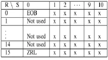
Huffman encode data i.e, the resulting quantised integer coefficients are then Huffman encoded to squeeze that extra bit of compression out of the image and convert to bit streams using the tables .Each scan is Huffman coded, where AC coefficients are ordered as a 16×11 structure in the Huffman table. This structure is designed to serve 16 different R values I. and 11 values of S. This structure is shown in Table I. The Huffman code for each (R, S) pair in a scan is vent, followed by S additional bits to identify the actual value of the coefficient.

From Table I slot for R = 0, S = 0 is used for the EOB symbol, while R = 15, S = 0 indicates 15 consecutive zeros followed by a size 0( ZRL symbol) but the slots for S = 0 and R = 1 to 14 are reserved for the progressive format and are not used in baseline sequential format. We use those unused slots for signalling adaptive quantization to decoder thus making it JPEG standard-compliant.

In JPEG standard if S = 0 and R = 15 then 16 consecutive zeros are appended to the zig-zag scan in reconstruction. Otherwise the symbol is treated an EOB. All slots in Table I with S = 0 and R <= 15 are considered to be the same symbol i.e. EOB symbol.

[image:3.595.88.267.411.511.2]

Because of that, additional codes for different conditions may adopted by using the 14 unused slots in Table II.

III. APPLICATION OF DCTAND QUANTIZATION

The equation for the DCT between spatial domain and frequency domain is:

( ) ( ) ( ) ∑ ∑ ( ) ( )

( )

{ √

√ [( )

Where C(u,v) is the coefficient of the DCT matrix at point (u,v), f(x,y) is the spatial domain value at a coordinate (x,y) of the JPEG image array, N is the width and height of the image, and a(u), a(v) are normalization constants.

Algorithm 1: Applying DCT

Intput: Original image block of 8*8 Output: DCT coefficient matrix

Step 1: Dividing the image into 8*8 blocks provides another advantage to applying DCT. With set values of N, u &v, a standard DCT coefficient matrix can be constructed taking N=8.

Step 2: The DCT is designed to work an pixel values ranging from -128 to 127, the frequency domain block is subtracting 128 from each entry to level off

A=A-128.

Step 3: Now we can apply DCT to the image block by simplifying the transformation to matrix multiplication, as, B=CAC|

Where B, the frequency domain matrix, C is the DCT coefficient matrix and A is the 8*8 original frequency domain block of image.

This block matrix now consists of 64 DCT coefficients, cij, where i and j ranges from 0 to 7. The top left coefficient,c00,correlates to the low frequencies of the original image block .As we move away from c00,the DCT coefficients correlate to higher and higher frequencies of the image .As, human eye is more sensitive to low frequencies ,and results from the quantization step will reflect this fact.

Table I

[image:3.595.66.265.621.728.2]

Huffman table layout for baseline sequencing mode.

Table II

(4)

International Journal of Emerging Technology and Advanced Engineering

364

Varying level of image compression and quality are obtained through selection of specific quantization matrices .This enable the user to decide on quality levels ranging from 1 to 100,where 1 is the poorest image quality and highest compression and 100 is the best quality and lowest compression.

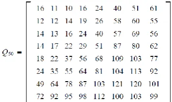
Subjective experiments uses the matrix developed by human visual system in the JPEG standard quantization matrix, with a quality level of 50 as show in Matrix I.

Algorithm 2: Quantization of matrix

Input: DCT Coefficient matrix Output: Compressed Image

Step 1: Another value of quality can be obtained by applying the equation as:

If quality level>50 then Q=Q50 * (100- quality level)/50

Else Q=Q50* quality level/50

Step 2: Quantization is achieved by dividing each element in the transformed image matrix B by the corresponding element in the quantization matrix Q, and the rounding to nearest integer value..

Ti,j=round(Bi,j/Qi,j)

A. Interaction with DC Prediction

A Potential complication with adaptive quantization is the dependence adjacent blocks. In baseline sequential JPEG, the DC coefficient of each block is coded as the difference from the corresponding value in the previously considered block in the scan. The prediction is reset by “restart” markers [6, pg 109], which may optionally be placed in the bit stream by the encoder. An adaptive quantization is used to predicting accumulate error when the DC coefficient is dequantized differently than that of it was quantized. The DC coefficient is unique in this respect though all other coefficients in a block are coded independently of adjacent blocks, therefore varying the Q matrix will has no effect.

We therefore confine the quantization change matrix H discussed above so that H(1; 1) = 1, which ensures that eX(1; 1) = X(1; 1) + EQ(1; 1). Alternatively, we may emit restart markers to reset the prediction on each block where the Q matrix changes. However, this adds to the output file size, which, while small, may be avoided by using the constraint.

B. Reduction of artifacts

It is well-known that JPEG compression results in at least two types of artifacts: 1) visible boundaries between 8X8 blocks; 2) ringing (Gibbs phenomenon) around edges. Although deblocking and de-ringing filters may be applied at the output to suppress those artifacts, it is obviously desireable to avoid the creation of the artifact. Adaptive quantization may be applied to this purpose. For example, if a given Q matrix produces both types of artifacts, we may apply a “smaller” matrix Q1 for smooth blocks, and a “larger” matrix Q2 for edge blocks, where Q2(u; v) > Q1(u; v). The identification of smooth vs edge blocks may be accomplished by noting whether the last non-zero coefficient occurs early or late in a zig-zag scan relative to a predetermined threshold as shown in figure 1.

Matrix I: Quality factor

[image:4.595.61.239.157.262.2]

Table III

Table of the Bit-coded values for DC Coefficients

Len gth

amplit

ude Code

1 -1,1 0, 1

2

-3,-2,2,3 00, 01, 10, 11

3

-7..-4,4..7

000, 001, 010, 011, 100, 101, 110,

111

4

-15..-8,8,15

0000, 0001, ……, 1111

5

-31..-16,16..31

00000, ……, 11111

Table V

Table of the Category and bit-coded values for AC Coefficients

Run/Length Code Length Code Word

0 / 0 (EOB) 4 1010

0 / 1 2 00

1/2 5 11011

(5)

International Journal of Emerging Technology and Advanced Engineering

365

IV. HUFFMAN TABLE MODIFICATION

Before storing all the coefficients of C are converted to bit stream Huffman coding takes advantage of redundancies – such as a list of numbers ending with a long list of zeros by inserting a new code in the place of a frequent combination of numbers. In JPEGs a common code signifying that the rest of the coefficients in a matrix are zero is EOB. The progressive Huffman table uses all of the slots, including the 14 slots for 1 <R< 14 for additional codes EOB1, : : :, EOB14. This allows up to 15 different Q matrices to be signalled.[3] The organization of a typical progressive table is shown in Table I taking the idea of Kakarala .

Algorithm 3: Modified Huffman Coding

Input: Compressed Image Output: Bit stream Code

Step 1: Application of differential coding using the mathematical representation of the differential coding is:

Diffi = DCi - DCi-1

We set DC0 = 0. DC of the current block DCi will be equal to DCi-1 + Diffi .Therefore, in the JPEG file, the first coefficient is actually the difference of DCs. The bit stream is calculated using the Table III and Table IV as for

DCi-1 DCi

One difference the bit stream is= (bit coded values of RUN, code word for size) together form a bit stream for the difference.

Same way all the differential coefficiences bit stream is calculated.

Example: Difference between blocks = 1 5 -9 -3

DIFF 1 5 -9 -3

Code from

table IV 1 101 0110 00

Code Length 1 3 4 2

Code Word

from table 2.3 010 100 101 011

OUTPUT: Final bit stream of DC coefficient is...0101100101101011001100

Step 2: After quantization and zigzag scanning, the one-dimensional vectors with a lot of consecutive zeroes is obtained. We can apply zero-run-length coding, which is variable length coding. We considered the 63 AC coefficients in the original 64 quantized vectors first.The notation (L,F) means that there are L zeros in front of F(run), and EOB (End of Block) is a special coded value means that if F is 0 and L is some value then ,the progressive Huffman table uses all of the slot , including the 14 slots for 1<R<14 for additional codes EOB1: : :,EOB14 as in Table II.

Step 3: The encoding method is quite easy and straight forward, For instance, the code (0,57) is 1111000 1111001 as in Table 2.2.The final bit stream is calculated .

Step 4: The difference is encoded with Huffman coding algorithm together with the encoding of AC coefficients.

Therefore, we may replace any of the 14 unused entries in Table II with additional codes for alternative conditions without disrupting a standards compliant decoder. The same is implemented for the ROI and the Original image.

V. IMPLEMENTATION OF REGION OF INTEREST

In ROI based image compression certain parts of the image are encoded with higher quality than others. This may be combined with scalability (encode these parts first, others later).Many of the image processing operations in IGOR can be selectively applied to a user defined region within the image.[7] This region is known as the region of interest or ROI. Many operations that support an ROI can execute significantly faster when the ROI is used to define a region that is much smaller than the full image. In particular, the ROI does not have to be rectangular or connected; it may consist of one or more disjoint Standard as defined earlier.

Algorithm 4: Implementation of ROI

To obtain number of ROI apply loop to the below steps:

Step 1: First crop the image for the region of interest.

Step 2: Apply all the three algorithms defined earlier to get the required amount of compression we obtain Quantized matrix of ROI(K(i,j)) .

[image:5.595.56.268.590.773.2]

Step 3: To get the target output ROI-JPEG join the original image Quantized image with the ROI quantized image by keeping the track of Xmin ,Ymin,width and height while cropping. Using the values and size of the new image(ROI) ie, row (M)and column(N).

Table IV

Table of the category and bit-coded values for DC Coefficients

Additional Code

Length(Category) Code Word

0 00

1 010

2 011

3 100

4 101

Diffi = DCi DCi-1

……….

(6)

International Journal of Emerging Technology and Advanced Engineering

366

W=Xmin+row-1 U=Ymin+column-1 T(Xmin:W,Ymin:U)=0; T(Xmin:W,Ymin:U)=K;

VI. EXPERIMENTAL RESULTS

The first results that we show here come from our experiments using a child image as the original image as shown in Fig 2(a).By applying DCT Algorithm , Quantization and Huffman coding i.e. Algorithm1 ,Algorithm2 and Algorithm3 to the Original image(Fig 2(a)) we obtain an compressed ratio(CR) of the image is 297.62 , when an quality of 1% is applied as shown in (Fig 2(b)). After applying decompression algorithm to the (fig 2(b)) we obtained an compressed image with Peak Signal Noise Ratio(PSNR) value of 17.42 as seen in (fig 2(c)).

Similarly the second results shown in fig 3 shows the results for the same child image (fig 3(a)) applying algorithm 1, algorithm 2 and algorithm 3 we get the compressed image with compression ratio of 12.98 when a quality of 95 % is applied to the (fig 3(a)) as shown in (fig 3(b)) and finally after applying decompression algorithm to (fig 3(b)) we obtain the restored image with PSNR value of 18.24 and obtain an image of the form shown in (fig 3(c)).

The next figures shows the experimental results of the same Child image by applying the ROI in different ways.ROI can be applied to any image according to the requirement of the user.

This paper only shows how the ROI works and the type of results we are obtaining if the ROI is applied. So the experiment only shows some of the results. The first experiment result is shown in fig.4 of two different qualities applied to the different halves of same image.

The second experiment result is shown in fig 5 with two qualities applied to same image by taking Face of the child as Region of interest. And finally we show the experiment results showing that not only two regions we can select but more than 2 we may select so the fig 6 shows that the eyes and mouth are the region of interest and the remaining image is the background with lesser interest.

Fig.2 Experiment result of document image of a Face .(a)Original face image.(b) DCT image with 1% Quality (c) Decompressed image of the original image with quality 1%

Fig.3 Experiment result of document image of a Face .(a)Original face image.(b) DCT image with 95% Quality (c) Decompressed image of the original image with quality

95%

Fig.5 Experiment result of document image of a Face .(a)face image with 1% quality decompressed image.(b) face image with 95% quality decompressed image (c) Combining both images with face as region of interest face with Quality 95% and Background with 1% quality

Fig.4 Experiment result of document image of a Face .(a)Original face image.(b) DCT image with 95% Quality and 1%quality (c) Decompressed image of the original image half

image with quality 95% and other half with 1% quality

Fig.6 Experiment result of document image of a Face .(a) face image with 1% quality decompressed image.(b) face image with 97% quality decompressed image (c) Combining

(7)

International Journal of Emerging Technology and Advanced Engineering

367

The experiment carried out taking two different qualities for the background and the ROI .The fig 4(a) contain the full image with Quality 1% which is taken as the background, the CR for this image is 297.62 and PSNR is 17.42.fig 4(b) is the restored image with quality 95% and the CR is 12.98 ,PSNR is 19.24 ,the final result we obtained in upper half with quality 95% and lower half with quality of 1% and the CR is 19.54 and PSNR value is 20.45.

The second experiment result is shown in fig 5 with two qualities applied to same image by taking Face of the child as Region of interest. And finally we show the experiment results with two different regions with quality of 1% and quality of 95%, we obtained the CR is 19.54 and PSNR value is 20.45. The fig 5 shows the experiments result by taking the face as region of interest. Fig 5(a) with Quality 1% taken as the background quality as previously calculated CR=297.62 and PSNR is 17.42 and Fig 5(b) shows the image with quality 95% with CR=12.98 and PSNR=18.24, so by combining both and taking face as the region of interest we obtained the fig 5(c) with CR=38.01 and PSNR=19.24.

The third experiment shows the result with two ROIs and two qualities 1% for background and 97% for ROIs (Mouth and Eyes). The fig 6(a) shows image with Quality 1% and fig 6(b) shows the image with quality 97% and CR=10.97,PSNR=17.57 , by combining both and taking mouth and eyes taken as the region of interest e obtained CR=200.62 and PSNR=17.57.

VII. CONCLUSION

In this project, we described an efficient method of image compression based on the idea of what is required and what is not in the image data, and there by applying the required amount of compression at different parts of the image. The user can select any part of image and can enter the required quality for compression, if the subject is more important than more quality to the subject is provided by the user and less to the background.

Otherwise, if the subject is irrelevant to user and background is important then more quality is provided to the background and less to the subject. By using this we can create images that are memory-efficient that contains only the required data from the JPEG file. The project can be extended to automatically detect the objects and apply the compression quality for the required objects. This can be applied for recognizing the faces and applying good compression quality on it. This work can be useful for detecting the defects on the leather samples.

REFERENCES

[1] G.K. Wallace, “The JPEG still picture compression standard,”

IEEE transactions on consumer electronics, Vol. 38, No. 1, Feb. 1992,pp.1-67

[2] Gonzalez, R.C. and R.E.Woods, “Digital image processing”, New

Jersey: Prentice Hall, pp.1-67, 2002

[3] Kakarala, R. ; Bagadi, R. TENCON “A method for signalling

block-adaptive quantization in baseline sequential JPEG”,IEEE Region 10 Conference;pp.1-67,2009

[4] Ken Cabeen and Peter Gent,Math, “Image Compression and

Discrete Cosine Transform”, College of Redwoods,pp.1-67,

[5] Po-Hong Wu, Ting-Yu Chen,“Advance Digital Signal

Processing-JPEG for Still Image Compression-Tutorial”,IEEE.pp.1-67,

[6] http://users.ecs.soton.ac.uk/srk/jpeg/JPEG.html [7] WY Wei - unioviedo.es

[8] W.B.Pennebaker,” Adaptive Quantization within the JPEG Sequential mode,” U.S.Patent 5,157,488,pp.1-67

[9] www-ee.uta.edu/.../Amee_Project_report

[10] http://www.wavemetrics.com/products/igorpro/imageprocessing/r oi.htm

[11] http://www.ams.org/samplings/feature-column/fcarc-image-compression

[12] http://www.ijmer.com/papers/Vol2_Issue4/FN2428292831.pdf [13] http://en.wikipedia.org/wiki/Image_file_formats#JPEG.2FJFIF;

Wikipedia