The problem and solutions in using delay functions with bifurcating flows in system dynamics models

The problem and solutions in using delay 

functions with bifurcating flows in system 

dynamics models

Dangerfield, BC and Fang, Y

Title

The problem and solutions in using delay functions with bifurcating flows 

in system dynamics models

Authors

Dangerfield, BC and Fang, Y

Type

Conference or Workshop Item

URL

This version is available at: http://usir.salford.ac.uk/292/

Published Date

2004

USIR is a digital collection of the research output of the University of Salford. Where copyright 

permits, full text material held in the repository is made freely available online and can be read, 

downloaded and copied for non­commercial private study or research purposes. Please check the 

manuscript for any further copyright restrictions.

The Problem and Solutions in Using Delay Functions with

Bifurcating Flows in System Dynamics Models

Yongxiang Fang 1,2 and Brian C. Dangerfield1

1_{Centre for O.R. & Applied Statistics, University of Salford, Salford M5 4WT, UK}

2_{School of Management, Harbin Institute of Technology, P.R.China, 150001}

Abstract

:

There is a special form of system dynamics model structure, involving the use of DELAY functions, or their algebraic equivalents, that can cause a computational error which the analyst may not be aware of. A negative level, normally impossible in the corresponding real-world dynamic system, results which reflects mass being created by virtue of the model error. Furthermore, employing a negative constraint to avoid a negative level being developed is not a proper solution. In this study, the solution of the problem is developed and demonstrated by means of a simple model.

Keyword: System Dynamics, Delay Function, Bifurcating Flows.

1 Introduction

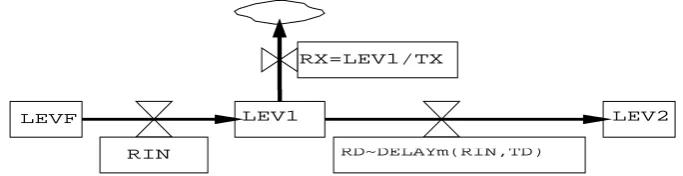
Developing a system dynamics model may require the use of a structure such as that shown in Figure 1. Here, the level variable LEV1 (simply denoted as L1 in the model listing) possesses one inflow RIN and two outflows RX and RD. RX is the rate that flows out of L1 and then exits the main flow. It is often directly proportional to L1. RD represents the rate that flows out of L1 and into level variable LEV2 (simply denoted as L2). In addition, RD is not directly related to L1, but rather to RIN by an mth

[image:2.595.123.465.414.502.2]

-order (m

≥

1) DELAY function. The tilde (~) character is used in figure 1 to represent not equivalence, but ‘similar to’.

Figure 1. Flow diagram for a category of system dynamics model structure

The structure described in figure 1 could well represent a fairly common model formulation. For instance, in modelling disease progression rates the flow RX could represent people dying from unrelated causes while the flow RD represents progression to the next stage of the disease. Also, in a model of a manufacturing process, RX could represent the flow out of sub-quality products whilst RD represents the quality finished products. In each case, the time constant on the flow RX (called TX) is likely to be somewhat larger than the corresponding time constant on RD (called TD).

As a fairly common model formulation, the structure shown as figure 1 may be used in many system dynamics models. An important issue for the analyst is that a computational error will be introduced if the structure is not dealt with properly. A mistake which is most likely to be made in formulating this model structure is simply ignoring the difference between the ‘~’ symbol and the ‘=’ symbol, then the main outflow RD is modelled as a mathematical DELAY function.

For example 1, suppose TX is given a value of 10 time units, TD is given a value of 5 time units and a third order delay is employed for RD. This kind of formulation may be modelled simply as (using the original system dynamics syntax):

L L1.K=L1.J+DT*(RIN.JK-RX.JK-RD.JK)

LEVF LEV1 LEV2

RX=LEV1/TX

N L1=0

R RX.KL=L1.K/TX

R RD.KL=DELAY3(RIN.JK,TD) C TX=10

C TD=5

However, unless an adjustment is made, the modeller using this formulation is in error. When the model is run (see below) there is a mass-balance problem in that L1 is eventually driven negative, a situation which is not normally allowable in a system dynamics model. (Modelling cash balances may be an exception to this statement but nonetheless the error would apply equally to that application.)

Strictly speaking there is a model formulation error created immediately by these equations. The DELAY function creates its own internal level(s) and, because of this, part of the input flows out twice: mass is created and the level (L1) can be driven negative.

In order to show the problem clearly a 3rd-order delay is used for RD as an example. It is convenient to simplify the inflow RIN(t) to be a single PULSE:

   

+ > <

+ ≤ ≤ =

DT t t t t

DT t t t DT t Rin

0 0 0

, 0 1 )

( (1)

An arbitrary choice of LENGTH has been made and the value of DT is sufficiently small given the assumed values for the time constants TX and TD. The demonstration program (again using the original system dynamics software syntax) is as follows:

* demonstration program 1 N TIME=STIME

C STIME=0 C DT=0.25 C LENGTH=50

R RIN.KL=PULSE(4,1.0,50)

L L1.K=L1.J+DT*(RIN.JK-RX.JK-RD.JK) N L1=0

R RX.KL=L1.K/TX C TX=10

R RD.KL=DELAY3(RIN.JK,TD) C TD=5

L CURIN.K=CURIN.J+DT*RIN.JK N CURIN=0

L CUOUT.K=CUOUT.J+DT*(RX.JK+RD.JK) N CUOUT=0

A CHECK1.K=CURIN.K-L1.K-CUOUT.K

A CHECK2.K=CURIN.K-MAX(L1.K,0)-CUOUT.K RUN MODEL ERROR AND MASS-BALANCE CHECKS

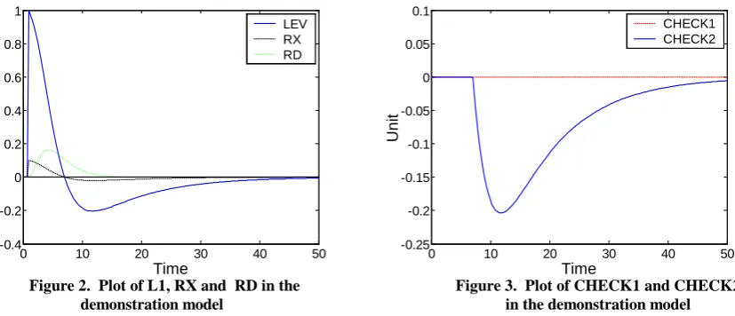
The plot of L1, RX and RD is shown as figure 2. Clearly L1 goes negative, which would normally be physically impossible.

The difficulty which can be caused by the structure in figure 1 is not well-addressed in the system dynamics literature. Nor, indeed, does any software package output a warning when such a structure is incorrectly formulated. A book by Coyle[1] (unfortunately with limited circulation) does touch on circumstances similar to the above (Problem 25: leaking model and Problem 29: two outputs from one delay). The leaking model in the book is formulated based on a cascading structure. However, there are no details and further discussions available.

similar to the

n

th-order delay”. The words “similar to” are crucial here for we have shown that, where side exit flows also appear from each level in the chain, then the result is indeed not equivalent to an

th

n

-order material delay, no matter whether the constituent delay constants are all equal or not.

0 10 20 30 40 50

-0.4 -0.2 0 0.2 0.4 0.6 0.8 1

Time

Un

it

[image:4.595.94.508.175.353.2]

LEV RX RD

Figure 2. Plot of L1, RX and RD in the demonstration model

0 10 20 30 40 50

-0.25 -0.2 -0.15 -0.1 -0.05 0 0.05 0.1

Time

Un

it

CHECK1 CHECK2

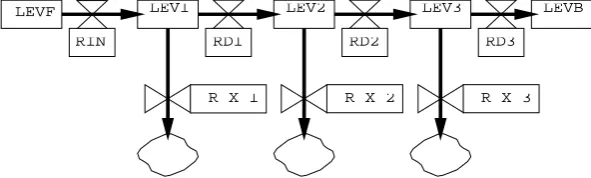
Figure 3. Plot of CHECK1 and CHECK2 in the demonstration model

As it has been shown in figure 2, a computational error will exist if the structure described by figure1 is not formulated correctly. However, the error is not easily identified by routinely used model testing techniques. For example, as part of the array of tests[3] which should be routinely applied to a model, a check for the conservation of matter (equivalent to a mass-balance test) is thought to be useful[4]. This is indicated especially where the flow(s) involve bifurcations, mergers or have an element of cycling, but problems can equally arise in a single source-sink flow. No resource should be unintentionally created or destroyed in a system dynamics model and the CHECK1 equation to verify this for any given resource flow will take the form:

CHECK1=SUMINFLOW-RELEVANT LEVELS-SUMOUTFLOW+ INITIAL VALUES FOR LEVELS (2) This should be zero, or the equivalent of zero given the floating-point accuracy on the computer, at all times.

However, the above mass-balance CHECK1 equation won’t pick up the error when a DELAYis used on one of the outflows. In order to pick up the error, a non-negative constraint must be applied to the level variable to create a second (and now revised) mass-balance check equation. It can be written as: CHECK2=SUMINFLOW-MAX(RELEVANT LEVELS,0)-SUMOUTFLOW+INITIAL VALUES FOR LEVELS (3)

It is necessary to state that the function of the equation CHECK1 is to test the mass-balance and the function of the equation CHECK2 is to pick up the error of having negative levels. A correct model should be able to pass both CHECK1 and CHECK2. Figure 3 shows the outcomes of CHECK1 and CHECK2 in the demonstration program 1. It shows that the formulation can pass the test given by the CHECK1 equation, but it cannot pass the test created by the CHECK2 equation. This means that a computational error arises from the formulation which is programmed in the demonstration program 1.

take a certain time before it manifests itself. This depends on both the dynamic behaviour of the model and the inflow to the model. It is difficult to know when a negative level will appear especially if the inflow is not simply a PULSE. For example, if the input flow is a STEP function, then level L1 in the demonstration program 1 will never be negative no matter how long a LENGTH is selected. Therefore, a model error may not be identified by CHECK1 and CHECK2 if the tests are not used properly.

2 Refining and illustrating occurrences of the model structure

In the real world, a large number of processes can be described by a model structure with bifurcating outflows where one represents the leakage and another the main outflow. ‘Leakage’ used here means flowing out of the process before completion of the desired process task. A leakage type outflow is commonly modelled as directly proportional to the source stock value and we use RX to represent it throughout this study. The main outflow is defined as leaving the process after having completed the desired process task and RD is used to represent it in this study.

A practical problem of this kind can be classified into two different categories according to the nature of task orientation in the process. In the first category, the purpose of the process is to transfer the input subject into a process output and the transformation takes a certain amount of time. In the second category, the process does not cause any change in the input subject, merely providing space for the input subject’s sojourn. How long the subject stays in the process does not depend on the process itself. In one extreme situation, the input subject can flow out of the process without any stay. In the opposite extreme situation, it may stay in the process for a very long time, indeed forever. For ease of description, we call the time required for input subjects to complete a process the ‘delay time’ and we call the time in which a subject actually stays in a process the ‘sojourn’ time. The delay time of a process is decided by the nature of the process. We call processes of the first category a ‘time-obligated process’ and name the second kind of process a ‘non-time-obligated process’.

One issue that should be emphasized is that the sojourn time in a time-obligated process is closely related to the delay time of the process. Although the sojourn time may be different between individual subjects, taking all individual subjects as a whole the mean sojourn time will be the same as the delay time. Moreover, this kind of process either has an infinite processing capability or, for any given inflow, its capability is large enough to handle all the individual subjects in the process simultaneously and independently. That is, the progression of an individual subject in the process is not affected by the status of any other individuals. In such a process, the output is governed by the inflow because the dynamic development of the process is “pushed” by the inflow. For a time-obligated process possessing such features a DELAY is a suitable function to model it. When a time-obligated process is associated with a leakage then the process should be fitted into the model structure addressed by figure 1. Two examples are given below.

Firstly, the situation which drew our attention to the problem[6]: HIV/AIDS patients who are being given Highly Active Antiretroviral Therapy (HAART). It is possible that this therapy will not remain efficacious indefinitely. Should it break down sometime in the future, patients might leave the state “on HAART”. At the same time, there will also be some patients who die from an unrelated cause, whilst they are receiving HAART. Due to the fact that the progression of disease between individual patients is developed simultaneously and independently, the sojourn time varies between different individual patients. Patients most likely leave the state “on HAART” at a rate governed by a high order delay of their assimilation onto HAART.

machining process, the side exit flow commonly exists, Therefore, the model structure in figure 1 is suitable for a machining process.

In contrast, the non-time-obligated process is totally different and it exists very commonly in production and business processes. Storing finished products in a manufacturer’s stock and storing goods in the warehouse of a supermarket are typical examples. In this situation, the input goods are just waiting there to be picked and no time is consumed in rendering the input goods becoming the goods that are ready to leave. There are usually two outflows in the process, one is a leakage which represents the discarding of damaged or degraded goods while the other represents qualify goods leaving the stock. It is obvious that the main outflow here is not dependent on the inflow, but dependent on the capacity of the next process linked to it -- the market (though the outflow is also constrained by the stock level). In an extreme situation, goods can go through the process without any delay if the stock level is too low to meet the demand. At the other extreme, the goods can stay in stock for a very long time, assuming they are not discarded, if there is no demand for them any more. The dynamics of a non-time-obligated process is driven by the ‘pull’ from the outflow. Therefore, the main outflow RD is not linked with the inflow. This kind of process cannot be fitted to the model structure in figure 1.

3 The existing methods and relevant problems

There are generally two methods proposed and used to formulate the structure shown in figure 1. The first method is to add a constraint to RD to keep its source level L1 non-negative. The application of this method is very easy. If we start from the demonstration program 1 and change the formulation of RD into the equation below, a formulation for model structure based on the method is obtained.

R RD.KL=MIN(DELAY3(RIN.JK,TD), L1.K/DT) (4)

The second method is to transfer the model structure in figure 1 into a cascade of stock-flows[1]. If an

[image:6.595.171.467.492.581.2]

nth order DELAY is involved in the model structure, then its corresponding cascading structure must have exactly n stages. Figure 4 presents the cascading structure transformed from the structure defined in figure 1 when the order of DELAY is 3. The correspondence of the variables between the two structures are: the RD in figure 1 corresponds the RD3 in figure 4, the RX in figure1 maps to the sum of RX1, RX2 and RX3 in figure 4 and the L1 in figure 1 matches LEV1+LEV2+LEV3 in figure 4.

Figure 4. The cascading structure transferred from the structure defined in figure 1 (n=3)

The first method is very simple and may be proposed by modellers who have only had a brief look at the problem. We encountered this model problem during the development of a system dynamics model for the HIV/AIDS epidemic and discussed it with a number of system dynamics experts, analysts and modellers. Most of them suggested adding a constraint to RD. Furthermore, the possibility of adding a constraint to the outflow RD has even been integrated as an optional feature in the modern system dynamics software package iTHINK. However, further investigation reveals this method does not provide a proper formulation of the model structure in figure 1.

LEVF

RIN

LEV1

RD1

R X 1 LEV2

RD2

R X 2 LEV3

RD3

[image:7.595.91.516.235.426.2]

This method focuses on avoiding the appearance of negative levels in a model and it works. However, the appearance of a negative level in demonstration program 1 is caused by a fundamental model error which, in the first place, distorts the process behaviour. Any method which only avoids the appearance of negative levels is not a proper solution of the underline model problem as the distortion in the process behaviour still exits. In order to show the model flaw in the formulation based on the first method, the demonstration program 1 is now run in an iTHINK environment where a constraint on RD has been automatically put into place and we name this demonstration 2. A point which should be mentioned here is that in iTHINK, DELAY is only used for a pipeline delay and a delay function with finite orders is represented by the SMTH function., For example, SMTH3 is the equivalent of DELAY3. The demonstration results are shown in figure 5.

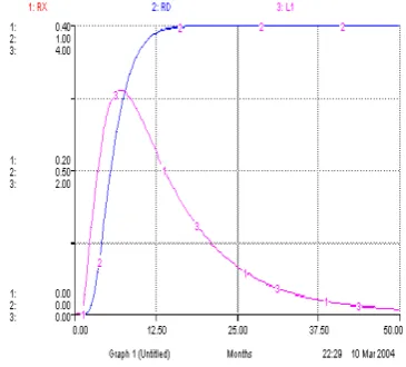
Figure 5 Outcomes of DEMO 2: A delay oriented process is truncated (single PULSE input)

Figure 6 Outcomes of DEMO 3, A delay oriented process becomes a through way (STEP input)

Though there is no appearance of negative levels in the model, it shows a truncation on the tail of RD. However, the truncation on RD is triggered by RD > L1/DT. If the value of L1 stays higher than the threshold, the truncation will never be triggered. Consequently, the outflow will be faster than it should be, the delay time will be cut down gradually and the dynamic behaviour of the system is then distorted. When the inflow is a STEP function and the process reaches near stable, the delay process will be distorted into a ‘wormhole’, that is the input will flow out of the process without any delay at all. We simply change the inflow in demonstration 2 from a PULSE into a STEP and call it demonstration 3. The results from demonstration 3 are presented in figure 6 which shows that the analysis is true.

The constraint put on RD here is used to prevent an outflow driving the stock value negative and it works well if RD is the main outflow of a non-time-obligated process. However, such a process cannot be fitted into the model structure shown in figure 1. For this reason it is no surprise that the first method does not provide an answer to the problem of formulating the model structure in figure 1.

Now, we turn to the second method: a cascading structure. This structure keeps RX always directly proportional to L1, while at the same time RD is an expansion of a high order delay. There is no difficulty in formulating this structure. However, the method has two weak points. The first one is very obvious: the structure transformation makes the model more complicated, especially when a high order DELAY function is involved.

[image:7.595.330.513.245.410.2]

time is unobservable. Unfortunately, in order to use the structure transformation method we need to know the functional delay time and, therefore, a method to derive the functional delay time from the actual delay time is required. Otherwise if we use the structure transformation method based on taking the actual delay time as the functional delay time, we will introduce a computational error.

4. Problem Solution

Expending the model structure in figure 1 into a cascade of stock - flows which make up the internal (hidden) elements is basically a correct approach. However, the barrier to its application is that the functional delay time is usually unknown. In order to overcome this barrier, a mathematical equivalent of the model transformation method is employed in this study. The solution based on the mathematical model provides a better and easier method to formulate the model structure presented in figure 1.

4.1 The mathematical model of the expanded leakage associated delay process

Firstly let an nthorder delay exist in the model structure in figure 1. Then the model structure can be expanded into a cascade containing n constituent stages. Then let the inflow RIN be a single PULSE which jumps at time point t = 0. Technically, this pulse input can be transferred into the initial value of

the level in the first stage of the cascade

l

₁, that is l1(0)=1 and at the same time RIN becomes constant

zero. We use

l

_i to represent the level variable at the

i

th stage of the cascade, Rd_ito represent the rate of the delay type outflow at the

i

thstage of the cascade, Txto represent the time constant for the leakage outflow at every stage of the cascade and T =Tf /n to represent the time constant for the delay type

outflow at every stage of the cascade, where Tf is the functional delay time of the process. Then the mathematical equations for the first stage can be written as:

) 3 . 5 ( ) 2 . 5 ( ) 1 . 5 ( / 1 ) 0 ( 0 1 1 1 1 ' 1       = = = + T l Rd l l l λ

The equations for the

i

th (i=2,3,...,n)stage can be written as:

) 3 . 6 ( ) 2 . 6 ( ) 1 . 6 ( / 0 ) 0 ( 1 '       = = = + ₋ T l Rd l Rd l l i i i i i i λ

In equation set (5) and (6)

λ

is a parameter related to Tx and T. It can be written as:

. ) 1 1 ( T Tx+ = λ (7)

4.2 The solution of the mathematical model

By solving the above equations, an expression of Rd_n can be obtained. Rd_n is actually the

equivalent of RD in figure 1. The expression of Rd_ncan be written as:

. )! 1 ( 1 t n n e T n t

Rdn −λ

−

−

= (8)

Furthermore, (8) is equivalent to:

. )!

1 (

1 n n 1 _t

n n n e n t T

Rd λ λ

In contrast, if the inflow is a PULSE input at time point t = 0, the output of an nth –order delay

function is defined as /( / )

1 )! 1 ( ) / ( n T t n f n f e n n T

t − −

− .It is clear that the first term of the right hand side of

equation (9) is a scale factor 1/(Tλ)n, the remaining part of the right hand side is an nth-order delay function when the inflow is a PULSE at the time point t = 0. That is, the output RD under the

mathematical formulation follows a rescaled nth-order delay function which is with a time constant n/λ. Let Ta = n/λ. This is the actual delay time of the process.

Let Kd represent the scale factor of the delay function and Kt represent the scale factor of the time constant of the delay, then Kd= 1/(Tλ)n and Kt = Tf /(n/λ). Substituting T =Tf /n and equation (7) into

them, the expressions for computing the two scale factors are obtained.

n x T n f T x T n d

K _

      ⋅ + ⋅ = (10)         ⋅ + ⋅ = x T n f T T n t

K x (11)

4.3 Applications of the solution

Based on the solution of the mathematical formulation of the model structure in figure 1, a correct and simple method for formulating a leakage associated delay process becomes available. Actually if the function delay time Tfand time constant for the leakage Tx are known, the main outflow RD in the model structure in figure 1 can be formulated as:

RD.KL=(1/(1+TF/(n*TX))**m)*DELAYn(RIN.JK,n/(n/TF+1/TX)) (12)

A great advantage of this solution is that it can be used in different situations when different knowledge about a practical process is available. Two major situations are discussed here.

Firstly, where the values for the functional delay time Tf and the percentage of output through the main flow Kd are known, for example a machining process in a production system. In this situation, the key is obtaining the value of Tx . Based on our solution, the value of Tx can be computed by equation (10) and then equation (12) can be used.

Secondly, where the values for the actual delay time Ta and the percentage of output through the main flow Kd are known. Patients progressing from one disease stage to another is an example, where observations can provide a ratio of patients who enter into the next disease stage (Kd) and the average sojourn time taken (Td). The time constant Tx and functional delay time Tf are not available. In this situation, the key point is to make the values of Tx and Tfbecome available. Taking equation (10) and (11) as an equation set, it only contains two unknown variables Tfand Tx . The values of the two time

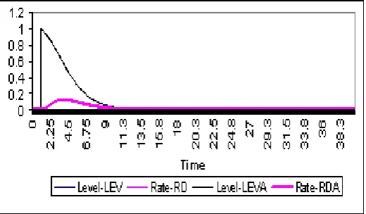
constants can be obtained from solving the equation set. Then equation (12) can be put into place. Finally, when Tx and Tfare known our solution is equivalent to the method which expands the delay function into a cascade of stock-flows. Demonstration 4 confirms this. In the demonstration, we retain the values for the constants in demonstration 1 and it is clear that TD= Tf . The demonstration program and results are shown below. The outcomes are plotted in figure 7 in which LEV results from the cascade method which is plotted exactly on top of LEVA which results from our solution. At the same time the RD (based on the cascade method) and RDA (based on our method) are exactly the same.

* Demonstration program N TIME=STIME

R RIN.KL=PULSE(4,1,40)

L LEV1.K=LEV1.J+DT*(RIN.JK-RX1.JK-RD1.JK) N LEV1=0

R RX1.KL=LEV1.K/TX R RD1.KL=LEV1.K*3/TD

L LEV2.K=LEV2.J+DT*( RD1.JK-RX2.JK-RD2.JK) N LEV2=0

R RX2.KL=LEV2.K/TX R RD2.KL=LEV2.K*3/TD

L LEV3.K=LEV3.J+DT*( RD2.JK-RX3.JK-RD3.JK) N LEV3=0

R RX3.KL=LEV3.K/TX R RD3.KL=LEV3.K*3/TD C TX=10

C TD=5

L LEV.K=LEV.J+DT*(RIN.JK-RX.JK-RD.JK) N LEV=0

R RX.KL=RX1.KL+RX2.KL+RX3.KL R RD.KL=RD3.KL

RUN the stage-split approach

L LEVA.K=LEV.J+DT*(RIN.JK-RXA.JK-RDA.JK) N LEVA=0

R RXA.KL=LEV.K/TX

R RDA. KL=DELAY3(RIN.JK/(1+TD/(3*TX))**3,TD/(1+TD/(3*TX))) RUN mathematical adjustment method

[image:10.595.170.430.433.585.2]

NOTE end of the program

Figure 7 Comparison of results from two methods

5 Further discussion and conclusions

In section 4, we developed a new method for formulating the model structure in figure 1. Based on the new solution the DELAY function in the model structure is rescaled by Kd and Ktwhich are defined by equation (10) and (11). Although the method provided a better and easier solution, some modellers may have doubts about it. Therefore we would like to present a few more arguments here.

being more general and precise, because in the real world a delay type process is commonly accompanied by leakages. The traditional method of using a DELAY function is an extreme example of the general method, where the scaling factors (Kd and Kt) are equal to exactly 1. That is, it can only be used in the situation where no leakage exists. Finally, the cascade-based method has been widely accepted, and this has been proved to be equivalent to use of a rescaled DELAY function. Therefore, there is no reason to oppose the new method.

The new method can also be supported by further analysis and tests. Firstly, further attention is focused on the equation (10). It is clear from the equation that three factors affect the allocation of the output between two outflows. When Tx increases or Tf decreases or n (order of delay) drops, the percentage distributed to outflow RD goes up. In the extreme, if Tx→∞, or Tf→ 0 this percentage will

→100% and the effects of the change in the order of the delay function is relatively much weaker. On the other hand we can see that if Tx→ 0, or Tf→ ∞, then Kd → 0. This is exactly the same as the real processes should behave.

Secondly, two further tests that can be conducted here are examining the value of Kd when the order of delay equals to 1 or infinity. For ease of discussion the form of equation (10) is changed equivalently into

n

x f T n

T d

K

−

    

  

⋅ +

= 1 (13)

When n = 1, the scale for the contributions of RD should be (1/Tf)/(1/Tf+1/Tx). It is exactly equivalent to the expression for Kd when n = 1. Equation (13) shows that when Txand Tf are fixed, the Kd

decreases as n increases (the order of the delay). When n tends to infinity, the delay function becomes a pipeline delay and the sojourn time of all subjects through the outflow RD will be identically Tf. Therefore, the scale for the contribution of RD should be exp(-Tf/Tx). In equation (13), Kd will also converge to the same value when n →∞. These tests support the new method presented here.

Thirdly, equation (11) regulates how the functional delay time of a process is scaled down by the associated leakage. It shows very clearly that the actual delay time will equal the functional delay time when the order of delay is infinite. Otherwise the two time constants are different. For our example (Tf = 10, Tx = 5 and n = 3) the scale factor is Kt = 6/7. This difference cannot be ignored. Therefore, the new method developed in this study provides a better and easier solution for formulating the model structure addressed in figure 1. We expect that this study will help modellers to employ the leakage associated delay model structure correctly in model formulation.

References:

[1] Coyle R. G. (1978) Equations for Systems, University of Bradford, UK.

[2] Sterman J. D. (2000) Business Dynamics. McGraw Hill/Irwin, New York.

[3] Forrester J. W. and Senge P. M. (1980). Tests for Building Confidence in System Dynamics Models. In: A.A. Legasto, J.W. Forrester and J. M. Lyneis (Eds.) System Dynamics. North-Holland: Amsterdam, pp 209-228.

[4] Coyle R. G. (1996) System Dynamics Modelling, Chapman and Hall, London.

[5] Forrester J. W. (1961) Industrial Dynamics, MIT Press, Cambridge, Mass.