International Journal of Emerging Technology and Advanced Engineering
Website: www.ijetae.com (
ISSN 2250-2459,
ISO 9001:2008 Certified Journal,
Volume 3, Issue 4, April 2013)
513
Voltage Control of AC-DC Converter Using Sliding Mode
Control
V. J. Sivanagappa
1, R. Ranjani
2, R. Suganya
3, K. Sumath
4, R. Yamuna
53,4,5
Student, Department of Electrical and Electronics Engineering
1,2Assistant Professor, Department of Electrical and Electronics Engineering
VIVEKANANDHA COLLEGE OF ENGINEERING FOR WOMEN, Tiruchengode, Namakkal – 637 205. India.
Abstract-- This paper deals with the concept of voltage control of AC-DC converter using sliding mode control. The main attribute of the sliding mode control is that converting a non-linear system into equivalent linear system. There are many types of controllers such as P, PI, PD, PID were used earlier. But this sliding mode control technique has simple and efficiency than the other method. The output voltage of the system is affected by electrical disturbance and mechanical disturbance. That disturbance is controlled by using sliding mode controller and buck converter. Where the simulation result is presented and it shows the fast dynamic response of the input variation, load disturbance and changes in reference value.
Keywords – Buck converter, Capacitor current, Output voltage, Phase controlled rectifier, Sliding mode control.
I. INTRODUCTION
The buck converter converts the fixed dc voltage into variable dc voltage in the range of less than the supply dc voltage level. That variable dc voltage is controlled by varying the firing angle of the converter switch. The buck converter output is non-linear and time variant system. So that, this converter can not applies for application of linear control technique. In order to design a linear control system we go for some control technique. The control techniques are P, PI, PD, PID and SLIDING MODE CONTROL. In these techniques, sliding mode control technique is only simple, robustness and fast dynamic response. Other techniques have some drawbacks like slow dynamic response, sudden increase in voltage level due to starting of motor, and tuning complexity. This sliding mode controller has more sensitive to input parameter variation, reference signal variation and load variation. These varying parameters are affect the motor and system efficiency. By using buck converter this variation is controlled. We use MOSFET to control the variation by controlling the firing angle of MOSFET.
This control technique is diagram of voltage control of ac to dc converter using sliding mode control technique is shown in fig.1. applied for small dc motor like 12V dc motor. The main ac source is converted into dc source by using phase controlled full wave rectifier. This dc source only fed to the buck converter and this is controlled by MOSFET. In this paper the mathematical model of buck converter and sliding mode controller are designed by using MATLAB/simulink. The block
Fig1. Block diagram of system.
II. MODELING OF BUCK CONVERTER
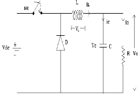
The principle of buck converter operation can be explained by fig.2. When the switch (sw) is closed, the Vdc
is directly connecting the load. The current flows through Vdc, switch (sw), filter inductor L, filter inductor C
International Journal of Emerging Technology and Advanced Engineering
Website: www.ijetae.com (
ISSN 2250-2459,
ISO 9001:2008 Certified Journal,
Volume 3, Issue 4, April 2013)
[image:2.612.57.294.145.320.2]514
Fig 2. Buck converter.
Where the ON period is given below,
When the switch (sw) is opened, the Vdc does not
directly connect to the load. The freewheeling diode is forward biased so that it starts conduct. This conduction is due to energy stored in the inductor. That energy is discharged when the switch is opened. This inductor current flows continuously through filter inductor L, filter capacitor C, resistor R and diode. This inductor current falls linearly until the switch is again closed. Where the OFF period is given below,
(2)
When the switch is in ON condition, the voltage equation can be derived as follows
The input voltage is given by,
Using Kirchhoff’s current law the inductor current iL is
given by,
When the switch is in OFF condition, the voltage equation is given by,
Where u=0
By using Kirchhoff’s current law, the inductor current iL
is given by,
Combining the equation 4 & 6 we get
(
)
Where
Combining equation 3 & 5 we get the value of
(
) (
)
Where
International Journal of Emerging Technology and Advanced Engineering
Website: www.ijetae.com (
ISSN 2250-2459,
ISO 9001:2008 Certified Journal,
Volume 3, Issue 4, April 2013)
515
Fig3. Mathematical model of buck converter.
III. SLIDING MODE CONTROL
The principle of sliding mode control is to force the system state to S=0 for any initial condition to attain stability. For any disturbances the system state is forced back to line S=0. For infinitely fast switching state the system will move along the line after some finite time. This motion is called sliding mode and this is ideal movement of the system. Where consider S is sliding mode function. The system state is buck converter state like ON & OFF state of switch. If the switch is in ON condition S>0 and the switch is in OFF condition S<0.
[image:3.612.50.294.141.357.2]In sliding mode, we have two modes like reaching mode and existing mode. At the initial stage the system can not reach the switching surface i.e. S 0. So that a control directed towards the sliding surface is called reaching mode. After the system attain the reaching mode it must stable in that condition S=0 is called existing mode. This existing mode is called sliding mode. The sliding surface is shown in fig.4
Fig 4. Sliding surface.
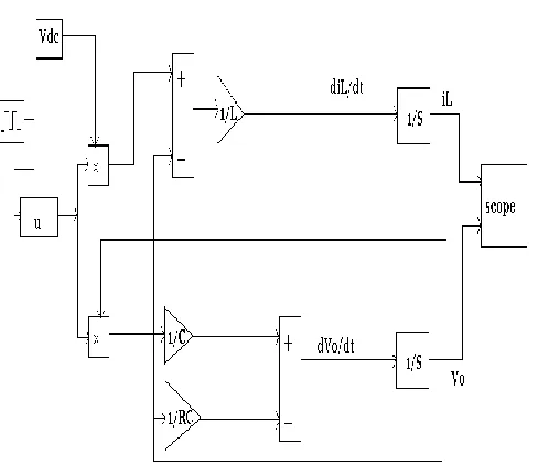
A. Design of sliding mode control
The design of sliding mode controller is shown in fig.5. X1 - Voltage error
X2 - derivative of voltage error.
Fig 5.sliding mode controller.
The value of X1 & X2 are given by,
(9)
[image:3.612.311.571.152.711.2]
International Journal of Emerging Technology and Advanced Engineering
Website: www.ijetae.com (
ISSN 2250-2459,
ISO 9001:2008 Certified Journal,
Volume 3, Issue 4, April 2013)
516
Using Kirchhoff’s law, the value of ic is given by,
(11)
Substitute equation (8) and in equation (11)
(12)
Normally the value of IC is given by,
Where
Then, the value of X2 and
is given by
,
(
)
(13)
(14) Substitute equation 9 & 10 in equ 14
,
(15)
[image:4.612.55.287.513.636.2]
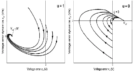
The graphical representation of individual substructures of the system with u=1 and u=0 for different starting(X1,X2)conditions are given in fig 6.
Fig 6. Phase Trajectory of the Switch Corresponding to a) u=1 and b) u=0
When u =1, the phase trajectory for any arbitrary starting position on the phase plane will converge to the equilibrium point(X1 = Vref – , X2 =0) after some finite
period. Similarly, when u=0, all the trajectories converge to the equilibrium point(X1 =Vref, X2 =0).
For slide mode controller, the switching state u can be determined from the control parameters X1 and X2 using
the switching function. The sliding function (S) is given by
(16) Where is sliding co-efficient
.
By enforcing S=0, a sliding line with gradient can be obtained. The purpose of this sliding line is to serve as a boundary to split the phase plane into two regions. Each of this region is specified with a switching state to direct the phase trajectory toward the sliding line. It is only when the phase trajectory reaches and tracks the sliding line toward the origin that the system is considered to be stable. i.e. X1=0 and X2 =0. If the phase trajectory is above the sliding
line(S=0), switch must be on so that the trajectory is directed toward the sliding line. Similarly, when the phase trajectory is at any position below the sliding line, switch must be off to maintain the trajectory on the sliding line. This forms the basis for control law.
To maintain on the sliding line Lyapunov’s second method to determine asymptotic stability must be obeyed. It is given by,
Slide mode controller requires the continuous monitoring of the parameters X1 and X2 for its control
Substitute the equation 9 & 13 in equation 16
(
)
Where k1 = 1/RC and k2 = - /C. The terms (Vref – Vo)
and ic are the feedback state variables from the buck
regulator that should be amplified by gain co-efficient k1
and k2 respectively. Normally capacitance is in the range of
microfarad, its inverse term will be significantly higher than and R. Hence, the gain co-efficient k1 and k2 become
International Journal of Emerging Technology and Advanced Engineering
Website: www.ijetae.com (
ISSN 2250-2459,
ISO 9001:2008 Certified Journal,
Volume 3, Issue 4, April 2013)
517
Fig7. Mathematical model of sliding mode controller.
B. Simulation result of sliding mode control
[image:5.612.49.295.139.306.2]The closed loop control is used to control the output voltage when the disturbances occur due to electrical disturbance and mechanical disturbance. This disturbance is rectified by sliding mode controller. The simulation result is shown in following figures.
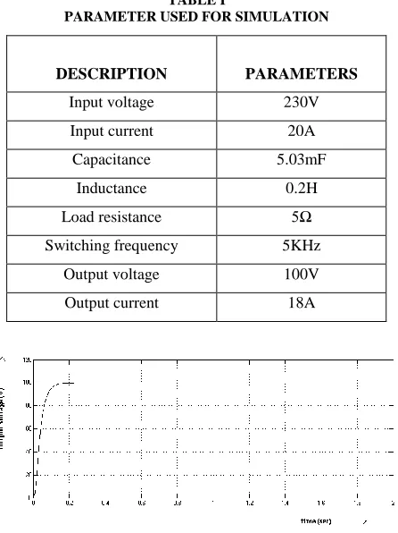
TABLE I
PARAMETER USED FOR SIMULATION
DESCRIPTION PARAMETERS
Input voltage 230V
Input current 20A
Capacitance 5.03mF
Inductance 0.2H
Load resistance 5Ω
Switching frequency 5KHz
Output voltage 100V
Output current 18A
[image:5.612.335.574.152.261.2]Fig 8.output voltage for step change in input voltage
Fig 9. Output current for step change in input voltage
Fig 10. Output voltage for change in load
Fig 11. Output current for step change in load
Figure 8 shows the simulation result of input voltage changes from 230V to 150V at the time of 1 sec. The output voltage has not have any disturbance.
Figure 9 shows the simulation result of input voltage change from 230V to 150V at the time of 1 sec. The output current has not have any disturbance.
[image:5.612.332.580.305.412.2] [image:5.612.58.281.407.705.2] [image:5.612.334.572.452.553.2]International Journal of Emerging Technology and Advanced Engineering
Website: www.ijetae.com (
ISSN 2250-2459,
ISO 9001:2008 Certified Journal,
Volume 3, Issue 4, April 2013)
518
Figure 11 shows the simulation result of load changes from 5Ω to 2.5 Ω at the time of 1 sec. The output current changes from 20A to 40A at the time limit of 0.04 sec. After that it reaches the steady state.
IV. CONCLUSION
This paper has the simulation result of sliding mode controlled buck converter. In these results are step changes in load and input voltage, for that output voltage and output current changes linearly within 1 sec. fro that result, the system is in stable and the system is under linear control by electrical and mechanical disturbance.
REFERENCES
[1] Zhang Yan, Changxi Jin, and Vadim I. Utkin, “Sensorless Sliding-Mode Control of Induction Motors”, ieee transactions on industrial electronics, vol. 47, no. 6, december 2000.
[2] Hanifi Guldemir, “sliding mode control of Dc-Dc boost converter”, Journals for applied sciences 5(3): 588-592, 2005.
[3] Siew-Chong Tan,Member, IEEE,Y.M.Lai, “ General Design Issues of Sliding-Mode Controllers in DC–DC Converters”, ieee transactions on industrial electronics, vol. 55, no. 3, march 2008 [4] WilfridPerruquetti, JeanPierreBarbot, “slidig mode control in
engineering”, Marcel Dekker,2002.