Wavelet Based Evolutionary Response of Multi Span Structures Including Wave Passage and Site Response Effects

1

_{Wavelet-Based Evolutionary Response of Multispan}

2

_{Structures Including Wave-Passage and}

3

_{Site-Response Effects}

1

4

_{Van-Nguyen Dinh}

; Biswajit Basu

; and Ronald B. J. Brinkgreve

5 _{Abstract:Stochastic seismic wavelet-based evolutionary response of multispan structures including wave-passage and site-response effects is} 6 _{formulated in this paper. A procedure to estimate site-compatible parameters of surface-to-bedrock frequency response function (FRF) by using} 7 _{finite-element analysis of the supporting soil medium is proposed. The earthquake energy content is represented by a composite power spectrum} 8 _{density function contributed by the surface-to-bedrock FRF and bedrock power spectra. A long span multisupport structure is subjected to} spa-9 _{tially varying differential support motions where the spatial-variability is represented by bedrock parametric coherency models and time-lags.} 10 _{In addition to the time-lags from wave-passage effects, the site-response effects from different soil conditions at the supports are characterized} 11 _{by frequency-dependent time-lags. In an illustrative case study, a three-span, two-dimensional hangar frame is analyzed using the proposed} 12 _{formulations. The time-lags resulting from site-response effects and computed by different FRFs show different variation in trends and} fre-13 _{quency content. The site-response effect is found to introduce additional frequency nonstationarity and leads to an increase in the frame} 14 _{responses but with slower attenuation in time.DOI:10.1061/(ASCE)EM.1943-7889.0000708.©2014 American Society of Civil Engineers.} 15 _{Author keywords:Seismic analysis; Amplitude and frequency nonstationary spatial variability; Site-response effect; Wavelets; Parametric} 16 _{frequency response function.}

17 _Introduction

18 _{The ground motions at a site are random processes attributed to the} 19 _{complex characteristics of the sources and paths of seismic waves.} 20 _{Moreover, they are apparently nonstationary in both amplitude and} 21 _{frequency from frequency-proportional velocities of seismic waves} 22 _{and from traveling paths consisting of soil layers having different} 23 _{properties. The structural responses underground motions are} con-24 _{sequently random and temporally and spectrally nonstationary, and} 25 _{they should therefore be stochastically represented by time-varying} 26 _{statistical quantities such as the evolutionary power spectral density} 27 _{function (PSDF). When statistical quantities representing ground} 28 _{motions (input) are given for evaluating stochastic structural} res-29 _{ponses (output), the input-output relations are needed. The random} 30 _{vibration theory is applicable only if the input is time-invariant. For} 31 _{time-varying inputs, wavelet techniques are suitable tools because} 32 _{they can provide a joint time-frequency representation simultaneously.} 33 _{Wavelet techniques have been used to formulate the input-output}

34 relations of single degree-of-freedom systems (Basu and Gupta

35

1998, 2000) and multiple degree-of-freedom systems (Basu and

36

Gupta 1997;Tratskas and Spanos 2003) where the input spatial-37 variation was excluded and proportional damping was assumed.

38 Earthquake-induced ground motions are spatially varying because

39 of four distinct phenomena: incoherence, wave-passage, attenuation,

40 and site-response effects (der Kiureghian 1996). The spatial-variation

41 of ground motions has pronounced effects on structures. Stochastic

42 input-output relations of multisupport structures subjected to spatially

43 varying ground motions have been formulated by using random

44 vibrations (Hao 1994;Loh and Ku 1995) where incoherence and

45 wave-passage effects are considered and the ground motions are

46 only nonstationary in amplitude. Dumanogluid and Soyluk (2003)

47 and Zhang et al. (2009) considered incoherence, wave-passage, and

48 site-response effects in their ground-motion spatial-variability models

49 and carried out stochastic analyses of long-span bridges whereas the

50 frequency nonstationarity of excitations was neglected. The

site-51 response effect was shown to contribute considerably to the

max-52 imum response amplitudes. However, the influence of site-response

53 effect on the frequency content of the responses of the bridge could

54 not be investigated.

55 A more general and realistic input-output relation has been

pro-56 posed by Chakraborty and Basu (2008) using a wavelet-based

frame-57 work in which the ground motions are nonstationary in both amplitude

58 and frequency, the excitation spatial-variation from the wave-passage

59 effect is considered, and the nonstationarity in both amplitude and

60 frequency of the output are evaluated. That work is extended in this

61 paper to include the compatible earthquake energy and

site-62 response effect of supporting soil media beneath the supports.

63 In the literature, by including a term in the coherency phase, the

64 site-response effect is considered in formulating complex coherency

65 functions (der Kiureghian 1996) and in simulating spatially varying

66 nonstationary ground-motion time histories (Zerva 2009;Konakli

67

and der Kiureghian 2012). While this approach is suitable for 68 ground-motion simulation, it faces a difficulty in spectral analysis of 1_{Postdoctoral Research Fellow, Dept. of Civil, Structural and}

Environ-mental Engineering, School of Engineering, Trinity College Dublin, Dublin 2, Ireland. E-mail: [email protected]; [email protected]

2_{Professor, Dept. of Civil, Structural and Environmental Engineering,}

School of Engineering, Trinity College Dublin, Dublin 2, Ireland (corre-sponding author). E-mail: [email protected]

3_{Associate Professor, Faculty of Civil Engineering & Geosciences, Delft}

Univ. of Technology, 2628 CN Delft, Netherlands; and Manager, PLAXIS bv, Computerlaan 14, 2628 XK Delft, Netherlands. E-mail: r.brinkgreve@ plaxis.nl

69 _{evolutionary responses. The direct use of a complex function is not} 70 _{feasible for the second-order moment of the stochastic responses} 71 _{because it is a real quantity. Instead, an alternative approach is} for-72 _{mulated in this paper to separately represent the lagged coherency and} 73 _{the phase. The site-response effect is proposed to be characterized by} 74 _{frequency-dependent time-lags. The wavelet-based spatial-variation} 75 _{model for ground motion to evaluate stochastic response incorporates} 76 _{parametric lagged coherency, wave-passage, and site-response effects} 77 _{in this paper.}

78 _{For simulating spatially varying nonstationary ground motions} 79 _{and analyzing structural responses, the earthquake energy content} 80_{2 has been generally characterized by stationary two-sided Kanai} -81 _{Tajimi PSDF (Hao et al. 1989;Chakraborty and Basu 2008) and} 82_{3 Clough-Penzien PSDF (Hao 1994; Deodatis 1996;Dumanogluid} 83 _{and Soyluk 2003; Zhang et al. 2009) among others. The} Kanai-84 _{Tajimi and Clough-Penzien PSDFs are most commonly used in both} 85 _{parameterization and simulation of seismic ground motions (Zerva} 86 _{2009). However, when using these spectra, the bedrock is assumed} 87 _{to be rigid and the parameters for the structure sites are not estimated} 88 _{from the specific geological profiles, but are empirically assumed.} 89 _{Because the dynamic properties of the soil medium vary horizontally} 90 _{from site to site, such description of PSDF is unable to represent the} 91 _{frequency and characteristic damping of the real soil conditions. The} 92 _{effect of soil layer thickness is also not accounted for, i.e., the natural} 93 _{period of a soil layer is proportional to its thickness (Kramer 1996).} 94 _{A thicker layer of soft soil may exhibit lower frequencies close to the} 95 _{dominant ones of the seismic waves and cause larger amplification} 96 _{of the propagating waves than a thinner layer would. To account} 97 _{for the thickness of soil deposit (i.e., the depth of the bedrock), the} 98 _{earthquake energy content at a site is represented in this paper by} 99 _{a composite PSDF contributed by the surface-to-bedrock frequency} 100 _{response function (FRF) and the bedrock power spectrum. A} pro-101 _{cedure to estimate site-compatible FRF parameters byfinite-element} 102 _{analysis (FEA) of the soil profile under each individual support is} 103 _{proposed in this paper and applied in the considered case study. This} 104 _{procedure overcomes some of the existing limitations by accounting} 105 _{for (1) soil property horizontal variation, and (2) effects of soil layer} 106 _{thickness in the FEA.}

107 Usingthe proposed representations of ground-motion spatial- 4

108 variation in “Representation of Parametric Coherency Model for

109 Ground Motions”and earthquake energy in“Site-Compatible PSD of

110 Ground Motions in Soil Medium on Elastic Bedrock,”the

wavelet-111 based stochastic models of spatially varying ground motions (input)

112 and seismic evolutionary responses of multispan structures (output)

113 are formulated in “Wavelet-Based Modeling of Spatially Varying

114 Ground Motions including Wave-Passage and Site-Response Effects”

115 and“Wavelet-Based Evolutionary Responses of Multispan Structures

116 Subjected to Differential Support Motions including Wave-Passage

117 and Site-Response Effects,” respectively (see also“Formulation

118 for Calculation of Evolutionary Responses”). “Wavelet Basis

119 Function”reviews an efficient wavelet basis function to be used in

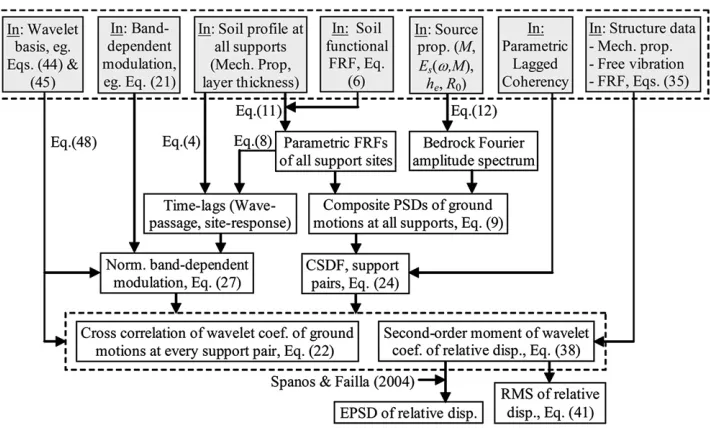
120 this paper. Aflowchart explaining the proposed methodology and

121 the relationship among the equations presented in this paper is

122 provided in Fig.1.

123 In the case study presented in“Numerical Example,”a

three-124 span, two-dimensional (2D) hangar frame supported on a

hori-125 zontally varying property soil layer and a thick elastic bedrock layer

126 is analyzed using the proposed formulations. The parameters of the

127 Clough-Penzien and Kanai-Tajimi FRFs compatible to the site

128 beneath each individual support are estimated. The stationary PSD

129 at each support is calculated by using the parametric Kanai-Tajimi

130 and Clough-Penzien FRFs. The stochastic processes corresponding

131 to these PSDs are used as orthogonal processes at different supports

132 for wavelet-based modeling of spatially varying ground motions

133 and for wavelet-based evolutionary response analyses of the frame.

134 The time-lags computed by using Kanai-Tajimi parametric FRFs

135 vary by a moderate amount around a higher frequency whereas

136 the time-lags computed by using Clough-Penzien parametric FRFs

137 vary dramatically around a lower frequency possibly stemming

138 from the additional lower frequency filter. Comparing with the

139 results in the case when only wave-passage effect is considered, the

140 site-response effect leads to an increase in wavelet-based root mean

141 squares (RMS) of the frame relative displacements with a slower

142 attenuation in time. The frequency content of such responses

143 exhibits stronger nonstationary and their instantaneous PSD peaks

144 are higher.

145 _{Representation of Parametric Coherency Model for}

146 _{Ground Motions}

147 _{The representation of ground-motion spatial variation by a proposed} 148 _{introduction of frequency-dependent time-lags for site-response} ef-149 _{fects and accounting for effects of incoherence and wave-passage} 150 _{is developed in this section.}

151 _{The coherency function characterizes the spatial variability of} 152 _{ground-motions in a frequency domain. Considering two supports} 153 _{randl, the coherency function is represented by the cross-spectral} 154 _{density function^S}

rlðvÞof the stationary parts of the ground motions 155 _{at the two supports, normalized by the square-root of the} corre-156 _{sponding PSDFs, i.e.,S}

rrðvÞandSllðvÞ, as (der Kiureghian 1996;

157 _{Zerva and Zervas 2002)}

grlðvÞ ¼ ^ SrlðvÞ

ffiffiffiffiffiffiffiffiffiffiffiffiffiffiffiffiffiffiffiffiffiffiffiffi SrrðvÞSllðvÞ

p (1a)

158 _{The PSDF of ground motion at a support is related to the FRF of the} 159 _{soil layer beneath that support, and the bedrock PSDF in Eq.(9).} 160 _{Eq.(1a)can be written in a complex variable form as}

g_rlðvÞ ¼ jg_rlðvÞjexp½iurlðvÞ (1b)

161 _{where the real term, jg}

rlðvÞj, 0#jgrlðvÞj#1, is the lagged co-162 _{herency characterizing the variation in space. In the literature,}

163 _jg

rlðvÞjhas been represented by common functions such as the ones 164 _{given, for example, by Harichandran and Vanmarcke (1986), Luco} 165 _{and Wong (1986), and Hao et al. (1989) . In this paper, the parametric} 166 _{coherency models are estimated by using FE-based seismic analysis} 167 _{of a geological soil medium model including the bedrock. The} 168 _{coherency phase urlðvÞ represents the difference in phase of the} 169 _{excitations at the two supports. When the wave-passage and} site-170 _{response effects denoted by the superscriptswpandsite, respectively} 171 _{are considered,urlðvÞis expressed as}

urlðvÞ ¼uwp_rl þusiterl ðvÞ ¼2vt wp rl þu

site

rl ðvÞ (2)

172 _{The use of representation in Eq. (1b) for spectral analysis of} 173 _{evolutionary excitations and structural responses faces the difficulty} 174 _{that the complex coherency cannot be directly introduced into any} 175 _{real-valued second-order moment quantity. To overcome this} dif-176 _{ficulty, the coherency phaseu}

rlðvÞis transformed into frequency-177 _{dependent time-lags as}

urlðvÞ ¼2v.trlðvÞ ¼2v

twp_rl þt_rlsiteðvÞ (3)

178 _{Consider a single soil layer under two surface sitesr and las} 179 _{shown in Fig. 2. The properties of the soil layer are horizontally} 180 _{varying. The propagation of seismic shear waves from the bottom to}

181 the top can be characterized by one-dimensional wave propagation.

182 The time-lag from the wave-passage effect in Eqs.(2)and (3)is

183 computed from the separation distancejrland the wave-propagation

184 velocitiesVrandVlbeneath supportsrandl, respectively, and is

185 given as

t_rlwp¼ 2jrl VrþVl

(4)

186 The site-response effect between sitesr and lis attributed to the

187 difference in phasesurand ulat the two sites as (der Kiureghian

188

1996)

usite

rl ðvÞ ¼ulðvÞ2urðvÞ ¼tan21

ImHlðvÞHrpðvÞ

ReHlðvÞHrpðvÞ

(5)

189 When the behavior of the soil column is dominated by itsfirst mode

190 or when the high-frequency components of the ground motion do

191 not have significant contribution to the structural responses, the

192 functional form of the FRF at a siteHsðvÞ,s5r,lin Eq.(5), can be

193 represented by the Kanai-Tajimi (K-T)filter function in Eq.(6)or

194 the Clough-Penzien (C-P) filter function in Eq.(7) (Clough and

195

Penzien 2003)

HsK-TðvÞ ¼

1þ2i§sðv=vsÞ

12ðv=vsÞ2þ2i§sðv=vsÞ

(6)

HsC-PðvÞ ¼H K-T s ðvÞ

v=vf

12v=vf

2_þ 2i§f

v=vf

(7)

196 In Eqs. (6) and (7), vs 5 soil characteristic frequency; and zs

197

5damping ratio. The frequencyvf and damping ratiozf used in

198 Clough-Penzien FRF, in Eq.(7), greatly attenuates the very low

199 frequency components. The frequency-dependent time-lag from the

200 site-response effect in Eq.(3)is given as

tsite_rl ðvÞ ¼21

vusiterl ðvÞ (8)

201 The maximum time-lags of ground motions at every support pairr

202 andl, from site-response effects, can be evaluated by substituting

203 v ðvs,r1vs,lÞ=2 for Kanai-Tajimi FRF or v ðvf,r1vf,lÞ=2

204 for Clough-Penzien FRF into Eq. (8). The time-lags twp_rl and

205 tsite

rl ðvÞ contributing to the coherency phaseurlðvÞ will be used

206 separately from the lagged coherency jg_rlðvÞj in the following

207 sections.

208 Site-Compatible PSD of Ground Motions in a Soil

209 Medium on Elastic Bedrock

210 In this paper, the geological profile consists of a soil layer on a very

211 thick elastic bedrock layer. The PSDF of ground motions at a

212 supportris related to that of bedrock motions by (der Kiureghian

213

1996)

SrrðvÞ ¼ jHrðvÞj2SbedrockðvÞ (9)

214 where HrðvÞ 5 FRF of the soil layer beneath support r; and

215 Sbedrock_{ðvÞ5PSD of bedrock. What follows later in the section is}

216 a proposed technique based on FE modeling of the soil medium to

217 estimate the parameters of this FRF represented by a parametric

218 form. The PSD of bedrock is expressed as

SbedrockðvÞ ¼ 1 TbedrockjF

bedrock_ðvÞj2 ₍₁₀₎

219 _{where T}bedrock _{5 stationary duration of the bedrock excitation} 220 _{stochastic process contributed by the earthquake source and the} 221 _{source-to-bedrock path (Trifunac and Brady 1975). The estimation} 222 _{of soil FRF parameters and the formulation of Fourier amplitude} 223 _{spectrum of motions at the top level of the bedrock (hereafter in short} 224 _{called the bedrock), F}bedrock_{ðvÞ, are presented in the following} 225 _sections.

226 _{Proposed Procedure to Estimate Site-Compatible} 227 _{FRF Parameters}

228 _{A procedure to estimate the FRF parameters of a single-layered soil} 229 _{column beneath a supportrby using FEA has been proposed. The} 230 _{soil column is modeled and analyzed using FEs. The software} 231 _{PLAXIS 2D (Brinkgreve et al. 2008) is used in this paper. The} 232 _{excitation is a white-noise acceleration uniformly applied at the} 233 _{bottom of soil layer. Assuming that the duration of the stationary} 234 _{motion at the bedrock level and at the surface level is the same, the} 235 _{unsmoothed absolute values of FRF of accelerations at the surface} 236 _{points with respect to the source (bottom) are computed from the} 237 _{Fourier amplitude ratio as}

jH~r,iðvkÞj ¼

jFsurface

r,i j jFbed

r,i ðvkÞj

; k¼1, . . .,Nv;i¼1, . . .,Npoints

(11)

238 _{whereNv 5number of discrete frequency intervals necessary} 239 _{around supportr; andNpoints5number of surface points considered} 240 _{around supportr. The value ofNvshould be chosen as a power of} 241 _{two to avoid zero-pad effects on fast-Fourier transform (Dinh and} 242 _{Basu 2012). The smoothed absolute values of FRF, jHr,iðvkÞj,} 243 _{k51, . . .,Nv, are obtained by averaging overNpointsthe number of} 244 _{surface points considered around supportr. The parameters of the} 245 _{FRF are estimated byfitting such smoothed absolute values to the} 246 _{functional form of the FRF, for example the Kanai-Tajimi spectrum} 247 _{in Eq.(6)or the Clough-Penzien spectrum in Eq.(7). The parametric} 248 _{fitting (nonlinear least square) in the softwareMATLABis used for} 249 _{this purpose. Model parameters (vs,z}

sfor Kanai-Tajimi FRF orvs,

250 _z

s,vf,zf for Clough-Penzien FRF) of the soil layer are obtained. 251 _{After comparing the statistical parameters (R-square,} root-mean-252 _{square error (RMSE)], afinal set of estimated model parameters and} 253 _{a parametric form jHrðvÞj of a soil column model at supportr is} 254 _{obtained for each FRF functional form. This procedure is repeated} 255 _{for each individual support having different local soil conditions.}

256 _{Fourier Amplitude Spectrum of Earthquake} 257 _{Bedrock Motions}

258 _{The Fourier amplitude spectrum of earthquake motions at bedrock} 259 _{is represented by using the stochastic seismic spectrum (Boore} 260 ₂₀₀₃₎

jFbedrock_{ðvÞj ¼C×E}

sðv,MÞ×GðRÞ×Pðv,RÞ×AðvÞ×DðvÞ (12)

261 _{where the scaling factor and the source spectrum are, respectively,} 262 _{expressed as}

C¼ ReVeFs

4pr₀V_s3₀ (13a)

Esðv,MÞ ¼v2M0 (

12ɛ 1þ ½v=vaðMÞ2

þ ɛ

1þ ½v=vbðMÞ2

)

(13b)

in which Re 5 radiation pattern; Ve 5 partition of total shear

263 wave energy into horizontal components;Fs 5constraint factor;

264 Vs0 5shear wave velocity;r0 5density of the source rock;va

265

5 lower-corner frequency of the source duration;vb 5

higher-266 corner frequency at which the spectrum attains one-half of the

high-267 frequency amplitude level; and ɛ 5 weighting parameter. The

268 moment magnitude M is mapped from the seismic moment M0 5

269 (dyn/cm). The geometrical spreading functionGðRÞis characterized

270 by empirical formulas well supported by data of distance range from

271 10 to 1,000 km with

R¼

ffiffiffiffiffiffiffiffiffiffiffiffiffiffiffiffi R2

0þh2e

q

272 whereR05epicentral distance; andhe5source depth.

273 For Eq.(12),Pðv,RÞ5path-dependent attenuation factor and is

274 dependent on propagation velocity;DðvÞ5diminution factor that

275 accounts for the path-independent attenuation of high-frequency

276 waveforms and can be represented by the k-filter; and AðvÞ

277

5amplification factor (which is approximated by the source/site

278 impedance ratio in a numerical scheme using the quarter-wavelength

279 approximation method).

280 Wavelet-Based Modeling of Spatially Varying

281 Ground Motions including Wave-Passage and

282 Site-Response Effects

283 A wavelet-based modeling of spatially varying ground motions

in-284 cluding wave-passage and site-response effects has been proposed

285 in this section. In wavelet analysis, a time seriesuðtÞis represented as

286 a composition of several time-localized shifted and scaled wavelets

287 (so-called the baby wavelets)ca,bðtÞof a basic waveletcðtÞ, where

c_a,bðtÞ ¼ 1ffiffiffiffiffiffiffi jaj p ct2b

a

(14)

288 The parameter b localizes the basis function at t5b and its

289 neighborhood, and the parameteracontrols the frequency content of

290 the basis function by stretching or compressing it. The discrete

291 wavelet transform has been used to simulate ground motions (Iyama

292

and Kuwamura 1999). Although the discrete wavelet transform is

293 the most efficient and compact, its power-of-two relationship in scale

294 fixes its frequency resolution (Gurley and Kareem 1999). Thus, the

295 continuous wavelet transform (CWT), which allows more closely

296 spaced scaling than the 2i_{relationship, is used in this paper. The}

297 CWT convolves the signaluðtÞwith a set of baby wavelets as (Basu

298

and Gupta 1997,1998,2000)

Wcuða,bÞ ¼ 1ffiffiffiffiffiffi jaj p

ð

uðtÞcpt2b a

dt (15)

299 where the asterisk 5complex conjugate. Eq. (15) gives the

lo-300 calized frequency information of uðtÞ around t5b. The value

301 Wcð×Þmaps afinite energy signal from the time domain to afinite

302 energy 2D distribution in the scale-translation domain.

303 A set of differential nonstationary ground motions €ugrðtÞ,

304 r51, . . .,Ns, atNssupports of a multispan structure is considered.

305 In practice,€ugrðtÞis an evolutionary random process and can be

€

ugrðt,vÞ ¼

ð ‘

2‘

Arðt,vÞeivtdGrðvÞ (16)

307 _{where A}r_{ðt,vÞ 5slowly varying time- and frequency-dependent} 308 _{modulation; anddGrðvÞ5orthogonal increment process associated} 309 _{with therth support such that}

E h

dGrðvÞdGpr

v9i¼0, vv9 (17)

E h

jdGrðvÞj2

i

¼SrrðvÞdv (18)

310 _{In Eq.(18),SrrðvÞ5two-sided PSDF of the stationary part of the} 311 _{random process, which has been formulated in Eq.(9). The} evo-312 _{lutionary random process in Eq.(16)can be transformed in wavelet} 313 _{domain by using Eq. (16), and the wavelet coefficients at a} dis-314 _{cretized scalea}

jcan be expressed as (Chakraborty and Basu 2008)

Wc€ugr

aj,b

¼ArjðbÞ

ð ‘

2‘

eivbdG~rðvÞ (19)

315 _{where orthogonal increment processdG~}

rðvÞsatisfies (Spanos and

316 _{Failla 2004)}

E h

dG~rðvÞdG~pr

v9i¼0, vv9 (20a)

E h

jdG~rðvÞj

2i

¼2pajjc^

vaj

j2SrrðvÞdv (20b)

The function ArjðbÞ represents the amplitude modulation for

317 _{€ugrðt,vÞ at a scale aj that can be the extended Shinozuka-Sato} 318 _{amplitude modulation (Shinozuka and Sato 1967) given as}

ArjðbÞ ¼arj

e2brjt2_e2l r jt

(21)

319 _{in whicha}r

j,brj, andgrj 5parameters of the amplitude modulation 320 _{for the ground motion at thejth band of frequency and at therth} 321 _support.

322 _{Multiplying both sides of Eq. (19) by the complex conjugate} 323 _{corresponding to another support l, as being carried out by} 324 _{Chakraborty and Basu (2008) and considering the} frequency-325 _{dependent time-lags from site-response effects, the cross} correla-326 _{tion of the wavelet coefficients of seismic ground motions at the two} 327 _{supportsrandland at a scaleajis}

EWc€ugr

aj,b

Wc€ugl

aj,b

¼ArjðbÞ

ð ‘

2‘ Arj

b2twp_rl 2trlsiteðvÞ

E

h

dG~rðvÞdG~plðvÞ

i (22)

328 _{where t}wp

rl 5 time-lag from the wave-passage effect; andtsiterl ðvÞ 329 _{5 frequency-dependent time-lag from site-response effects} pre-330 _{sented in Eqs.(4)and(8); and}

E h

dG~rðvÞdG~plðv9Þ

i

¼0, vv9 (23a)

E h

dG~rðvÞdG~plðvÞ

i

¼2pajj^c

vaj

j2SrlðvÞdv (23b)

331 The modulus of the cross-spectral density function between the

332 ground motions at two supportsrandlis written from Eq.(1a)as

SrlðvÞ ¼ j^SrlðvÞj ¼ jgrlðvÞj

ffiffiffiffiffiffiffiffiffiffiffiffiffiffiffiffiffiffiffiffiffiffiffiffi SrrðvÞSllðvÞ

p

(24)

333 In this paper, the earthquake energy transmitted to each supportr

334 is completely represented by its stationary PSDFSrrðvÞin Eq.(9).

335 Thus, the energy of the modulation must be unit-normalized before

336 convoluting with the power spectral densities in Eq.(19). The energy

337 content,IA, of a frequency-dependent modulation before

normal-338 izingAðt,vÞis given by

IA¼

ðT 0 ð ‘ 0

Aðt,vÞ2dvdt¼ P Nv

k51 PNt

n51

Aðtn,vkÞ

2

Dv×Dt (25)

339 The energy content is expressed in a band-dependent form as

IA¼P ma

j51 (

N_vj P Nt

n51

AjðtnÞ

2 )

Dv×Dt (26)

340 wherema5number of frequency bands;Nvj 5number of discrete

341 frequencies injth band; andNt5number of time intervals. Hence,

342 the unit-energy normalized amplitude modulation at a band j is

343 given by

AjðtnÞ ¼ AjðtnÞ

ffiffiffiffi IA

p (27)

344 Wavelet-Based Evolutionary Responses of

345 Multispan Structures Subjected to Differential

346 Support Motions Including Wave-Passage and

347 Site-Response Effects

348 Formulation for Calculation of Evolutionary

349 Responses

350 A formulation for calculating the evolutionary response including

351 wave-passage and site-response effects is derived in this section.

352 Consider a structure havingN degrees of freedom (DOFs) andNs

353 supports subjected to spatially varying excitation-time histories

354

€

ugrðtÞ,r51,. . .,Ns. The structure is modeled in a FE framework

355 leading to a discrete dynamical system model. Using the consistent

356 mass matrix approach and an assumption that the effect of the entire

357 velocity-damping coupling is negligible in comparison with that of

358 the inertia, the motion equations of the structure is given by (Clough

359

and Penzien 2003)

M€uþCu_þKu¼2MEþMg

€

ug (28)

360 whereuðtÞ5displacement vector relative to the support motions;

361 M5systemN3Nmass matrix;C5N3Ndamping matrix; and

362 K5N3N stiffness matrix. In Eq.(28), theN3Nsinfluence

co-363 efficient matrixE, whosekth column represents the displacements at

364 the unconstrained DOF when a support DOF is displaced by a unit

365 amount while all other support DOFs remainfixed, is expressed as

366 E5 2K21_K

g. TheN3Ns matrices Mg and Kg account for the

367 coupling of the inertia and stiffness between structural DOFs and

€

ug¼

D

€

ug1ðtÞ. . . €ugNsðtÞ ET

369 _{Using modal transformationy5Fz, wherey5hu u_ i}T_andF 370 _{5complex 2N32Neigenvector for the nonproportional damping} 371 _{case, andy[uandF5realN3Neigenvector for the proportional} 372 _{damping case, the uncoupled form of Eqs.(28)for the two damping} 373 _{cases are, respectively (Chakraborty and Basu 2008)}

_

zkþgkzk¼ P Ns

r51 xr

k€ugrðtÞ, k¼1, . . ., 2N (29)

€

zkþ2hkvk_zkþv2kzk¼ P Ns

r₅1 xr

k€ugrðtÞ, k¼1, . . .,N (30)

374 _{In Eqs.(29)and(30),z}

k5kth modal component of the generalized 375 _{coordinate vector z; and the right-hand-side load 5 sum of kth} 376 _{modal earthquake load over all supports, withx}r

k representing the 377 _{kth modal excitation factor at supportr. In Eq.(29),g}

k5complex 378 _{modal stiffness for the nonproportional damping case. In Eq.(30),} 379 _{vk 5modal frequency for the proportional damping case; andh}

k 380 _{5damping ratio for the proportional damping case.}

381 _{Transforming Eqs. (29) and (30) by a chosen wavelet basis}

382 _c

a,bðtÞ and using Eq. (19) and the relations ∂=∂b½Wczkðaj,bÞ 383 _{5Wcz_}

kðaj,bÞand∂2=∂b2½Wczkðaj,bÞ5Wc€zkðaj,bÞgives

∂ ∂bWczk

aj,b

þg_kWczk

aj,b

¼ PNs

r51 xr

kArjðbÞ

ð ‘

2‘

eivbdG~rðvÞ

(31a) ∂2

∂b2Wczk

aj,b

þ2hkvk∂

∂bWczk

aj,b

þv2

kWczk

aj,b

¼PNs r51

xr kA r jðbÞ ð‘ 2‘

eivbdG~rðvÞ (31b)

Solving Eqs. (31a)and (31b)(which resemble the equations of 384_{6 motion in wavelet domain) by using Duhamel’sintegral gives}

Wczk

aj,b

¼PNs

r51 xr

k

ð þ‘

2‘ M_rk

jðv,bÞe ivb_dG~

rðvÞ (32)

385 _where

Mkrjðv,bÞ ¼ ðb

0

hkðb2tÞArjðtÞeivðt2bÞdt (33)

386 _{Using time-localization aroundt5bof the wavelet transform and} 387 _{the less oscillatory nature of the band-dependent envelope function} 388 _Ar

jðtÞ compared with the unit impulse response function hkðtÞ, 389 _{Eq.(33)can be approximated as}

Mrkjðv,bÞ A r jðbÞ

ðb

0

hkðb2tÞe2ivðb2tÞdtArjðbÞHðvÞ (34)

390 _{whereHkðvÞ5conventional frequency-response function in thekth} 391 _{mode, which is given for the nonproportional and proportional} 392 _{damping cases in the respective equations}

jHkðvÞj ¼ 1 ivþgk

(35a)

jHkðvÞj ¼ 1

v2

k2v2þ2hkvkiv

(35b)

Taking wavelet transform of the modal transformation gives

Wcup

aj,b

¼ PNd

k51

Fp,kWczk

aj,b

(36)

393 whereWcupðaj,bÞ5wavelet coefficient of relative displacement at

394 pth DOFs; andNd5number of modes considered. Multiplying both

395 sides of Eq.(36)by its complex conjugate and applying expectation

396 operator gives the second-order moment of the relative displacement

397 alongpth DOF as

E h

W_c2up

aj,b

2i_¼ PNd

k₅1 PNd m₅1

Fp,kFp,mE

h W_cpzk

aj,b

Wczm

aj,b

i

(37)

398 Using the expressions ofWczkðaj,bÞand Wczmðaj,bÞin Eqs.(32)

399 and (33) and the cross correlation of the orthogonal incremental

400 processes in Eq.(23b), while considering the frequency-dependent

401 time-lags from site-response effects, Eq.(37)is simplified as

E h

W_c2up

aj,b

2i_¼PNd

k₅1 PNd

m51

2Fp,kFp,mP Ns

r51 PNs

l₅1 xr kx l mA r jðbÞ ð ‘ 0 fjðvÞdv

(38)

402 where

fjðvÞ ¼2pajA l j

h

b2t_rlwp2trlsiteðvÞ

i

.jHkðvÞj2SrlðvÞ c^

ajv 2

(39)

403 The terms Ar_jðbÞand Al_jb2twp_rl 2tsite

rl ðvÞ

5unit-energy

normal-404 ized amplitude modulations for €ugrðtÞ and €uglðtÞ at a scale j,

re-405 spectively. By using the second-order moments obtained from

406 Eq.(38), theEPSD of the relative displacement alongpth DOF can be 7

407 estimated (Spanos and Failla 2004).

408 Based on the time-lags considered, for seismic waves already

409 arrived at supportr but yet to arrive at support l, the modulation

410 intensity at the latter support should be zero, i.e.

Alj

b2twp_rl 2tsiterl ðvÞ

¼0 if b,t_rlwpþtsiterl ðvÞ (40)

411 The instantaneous mean-square value of a time-dependent process

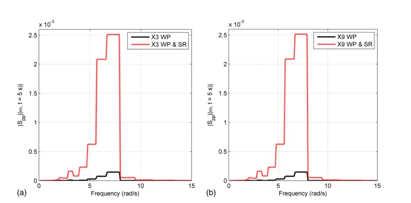
412 (Basu and Gupta 1998) is used to compute that of the relative

413 displacement along thepth degree of freedom as

E h

u2_pðtÞi t5bi

¼KP ma

j E

h Wc2up

aj,bi

2i

aj

(41)

414 where the termK is expressed as

K ¼s221

4pCcs (42)

415 In Eq.(42),s5parameter for discrete representation of the scale

Cc¼ ð þ‘

2‘ jc^ðvÞj2

v dv, ‘ (43)

417 _{Wavelet Basis Function}

418 _{Although in theory the proposed stochastic seismic evolutionary} 419 _{response is applicable for any wavelet basis function satisfying the} 420 _{admissibility criterion in Eq.(43), the choice of the basic function is} 421 _{important for the efficiency and accuracy in computation. Besides,} 422 _{the analysis resulted from CWT relies heavily on the scale} dis-423 _{cretizations and the selected frequency range (Kijewski-Correa and} 424 _{Kareem 2006). Several wavelet basis functions were shown} ad-425 _{vantageous in characterizing ground motions such as the Mexican} 426 _{hat wavelets (Zhou and Adeli 2003) and harmonic wavelets (Spanos} 427 _{et al. 2005). Tratskas and Spanos (2003) modeled the nonstationary} 428 _{base-excitations and estimate the stochastic evolutionary responses} 429 _{by using harmonic wavelets. Harmonic wavelets were also used by} 430 _{Spanos and Kougioumtzoglou (2012) to compute statistically} lin-431 _{earized evolutionary responses of nonlinear oscillators subject to} 432 _{stochastic excitation. The modified Littlewood-Paley (MLP) basis} 433 _{function (Basu and Gupta 1998) is used in this paper because it} 434 _{provides high accuracy in spectral analysis (Spanos and Failla 2004)} 435 _{and advantages in numerical computation by enabling energy} com-436 _{putation of any signal with nonoverlapping frequency bands. The} 437 _{MLP wavelet basis pair in time and frequency domain is given by}

cðtÞ ¼ 1

p ffiffiffiffiffiffiffiffiffiffiffiffiffiffiffiffiffiffiffiffiffiffiffi2F1ðs21Þ

p .sinð2pF1stÞ2sinð2pF1tÞ

t (44)

jc^ðvÞj ¼ ffiffiffiffiffiffiffiffiffiffiffiffiffiffiffiffiffiffiffiffiffiffiffiffiffiffi1 4pF1ðs21Þ

p , F1#

_2pv # sF1

¼ 0 otherwise

(45)

438 _{where F1 5 initial cutoff frequency of the mother wavelet. If} 439 _{F150:5 Hz, Eqs.(44)and(45)are reduced to the original forms of} 440 _{MLP basis function (Basu and Gupta 1998) as}

cðtÞ ¼ 1 ppffiffiffiffiffiffiffiffiffiffiffiffis21.

sinðpstÞ2sinðptÞ

t (46)

j^cðvÞj ¼ ffiffiffiffiffiffiffiffiffiffiffiffiffiffiffiffiffiffiffiffiffi1 2pðs21Þ

p , p #jvj# sp

¼ 0 otherwise

(47)

441 _{The scaled Fourier transform is}

jc^vaj

j ¼ ffiffiffiffiffiffiffiffiffiffiffiffiffiffiffiffiffiffiffiffiffiffiffiffiffiffi1 4pF1ðs21Þ

p when2pF1 aj

#jvj#2pF1s aj

¼ 0 otherwise

(48)

442 _{The admissibility criterion coefficient,Cc, in Eq.(43)becomes}

Cc¼ 1

2ðs21Þp ð þ‘

2‘ 1

jvjdv¼2ðsln2s1Þp (49)

443 _{It is noted by Basu and Gupta (1998) that fors52}1=n_{,n$4 is} 444 _{found reasonable, based on investigations on several ground motions}

445 recorded. However, because a small value ofs leads to increased

446 computational effort, a value ofs521=4_{has been chosen (Basu and}

447

Gupta 1998,2000;Spanos and Failla 2004). A higher value ofscan 448 also be chosen in the case of ground motion with relatively smooth

449 Fourier spectra.

450 Numerical Example

451 An application of the proposed theory and derived formulations in

452 this paper relating to evolutionary response of structures with

wave-453 passage and site-response effects is presented in this section. To

454 illustrate the wave-passage and the site-response effects on the

455 stochastic evolutionary responses, multispan structures that exhibit

456 considerable vertical and horizontal responses should be examined.

457 A three-span 2D frame of a hangar shown in Fig. 3 is therefore

458 considered. The cross-sectional area and moment of inertia of the

459 columns areAc51:2 m2andIc50:144 m4, respectively; and those

460 of the beams areAb52:0 m2andIb50:667 m4, respectively. The

461 frame material parameters are elastic modulusEb52:031011N=m2,

462 Poisson rationb50:29, mass densityrb57,860 kg=m3, and the

463 modal damping ratios for thefirst two modes arez15z250:02. The

464 firstfive natural frequencies of the frame are 6.72, 10.02, 12.07,

465 15.67, and 33:96 rad=s. A geological profile of the area beneath the

466 supports is shown in Fig.3and the data is presented in Table1. An

467 earthquake is assumed to occur with the moment magnitudeM55:5,

468 source depthhe520 km, and epicenter distanceR05100 km from

469 the bridge.

470 Using the procedure presented in“Site-Compatible PSD of

471 Ground Motions in a Soil Medium on Elastic Bedrock,”four soil

472 models representing the sites beneath four supports are analyzed by

473 FEs using PLAXIS 2Dwhere each soil domain is modeled with

474 dimensions 100350 m. Fine meshes are used for discretization of

475 the FE model with an automatic mesh generation scheme. Nine

476 surface observation points (Npoints59) located around the model

477 centerline have been chosen. The model domain width is chosen as

478 large as 100 m to reduce the effect of reflected waves at the vertical

Fig. 3.Three-span frame subjected to spatially varying ground motions and geological profiles beneath the supports; 3, 6, 9, and 14 are the observation points

Table 1.Propertiesof Soil Layers, Bedrock, and Source Rock ₁₀

Soil column EðMN=m2_{Þ v rðkN=m}3_{Þ V} sðm=sÞ

1 24.6 0.25 17.9 73.42

2 40.6 0.23 19.2 91.81

3 21.6 0.22 18.2 68.89

4 35.6 0.24 18.8 86.53

Bedrock 3,000 0.25 2,500 565.68

Source rock 70,533 0.23 2,800 3,200

479 _{boundaries on the observation points. A linear elastic soil model has} 480 _{been used for analysis. For generation of the FRFs,Nv51,024 has} 481 _{been chosen. The estimated parameters of Clough-Penzien and} 482 _{Kanai-Tajimi FRFs compatible to the sites beneath the supports are} 483 _{shown in Tables 2 and 3, respectively. In these tables,R-square} 484 _{stands for coefficient of determination and RMSE (standard error).} 485 _{The estimation of parameters for Clough-Penzien spectrum is better} 486 _{because its RMSE values are smaller andR-square values are larger} 487 _{and .0:5.}

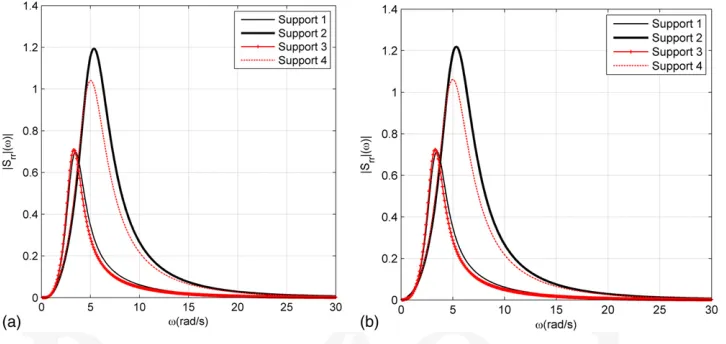
488 _{The stationary PSDs at the supports calculated by Eq.(9)using} 489 _{parametric Kanai-Tajimi FRF and Clough-Penzien FRF are shown} 490 _{in Figs. 4(a and b), respectively. The stochastic processes} corre-491 _{sponding to these PSDs are used as orthogonal processes at different} 492 _{supports for wavelet-based modeling of spatially varying ground} 493 _{motions employing Eq. (22) and for wavelet-based evolutionary} 494 _{response analyses of the frame employing Eq.(38). The variation of} 495 _{frequency-dependent time-lags between the left support and other} 496 _{supports from site-response effects calculated by using Eq.(8)are} 497 _{shown in Figs.5(a and b). The time-lags computed by using} Kanai-498 _{Tajimi parametric FRF vary by a moderate amount around the}

499 frequency of 4 rad=s whereas the time-lags computed by using

500 Clough-Penzien parametric FRF vary dramatically around a lower

501 frequency of 1 rad=s. Thisfluctuation in the time-lags in the

Clough-502 Penzien FRF case around a lower frequency may have resulted from

503 the additional lower frequencyfilter [Eq.(7)], which in some cases

504 may be a more realistic representation. The Clough-Penzien FRF is

505 therefore used in the computation for structural responses in the

506 following example even though the Kanai-Tajimi FRF could have

507 been used in the computation with equal ease. For Clough-Penzien

508 FRF, the time-lag peaks of ground motions at support pairs 1 and 2, 1

509 and 3, and 1 and 4 are∼2:1, 3.5, and 2.3 s, respectively. Each peak

510 occurs approximately around the averagevf(see Table3) of the soil

511 columns below the two corresponding supports.

512 The influence of site-response effects on the amplitude and

fre-513 quency nonstationarity of the frame-relative displacement responses

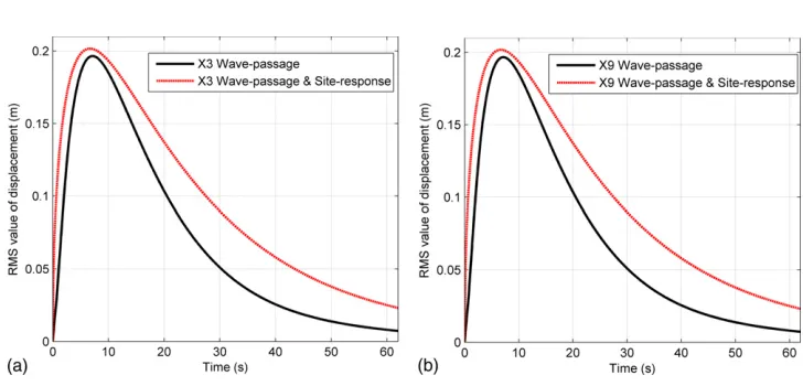
514 has been examined. Figs.6(a and b)show the RMS values of the

515 relative vertical displacement at the midpoints of the left span and the

516 midspan, respectively calculated by using Eq.(41). When the

wave-517 passage effect is considered alone, the RMS values decrease and

518 attenuate faster in time than those when both wave-passage and

site-519 response effects are considered. Similar influence of site-response

520 effects on the relative horizontal displacements at the top of thefirst

521 and the second columns can be observed in Figs.7(a and b),

re-522 spectively. The site-response effects are also shown to alter the

523 amplitude nonstationarity of frame displacements. The increase in

524 the response amplitude nonstationarity from the site-response effect

525 can be evaluated from Figs.6and7. The ratios of the increase in

526 average RMS displacement from the site-response effect, to the

527 average RMS displacement from the wave-passage effect, for the

528 nodes Y6, Y14, X3, and X9 are 41.8703, 42.3704, 39.7965, and

529 39.7949%, respectively.

530 The EPSDs of the relative vertical displacements at the midpoints

531 of the left span and the midspan using the parametric

Clough-532 Penzien FRF and Eq. (38) are shown in Figs. 8 and 9,

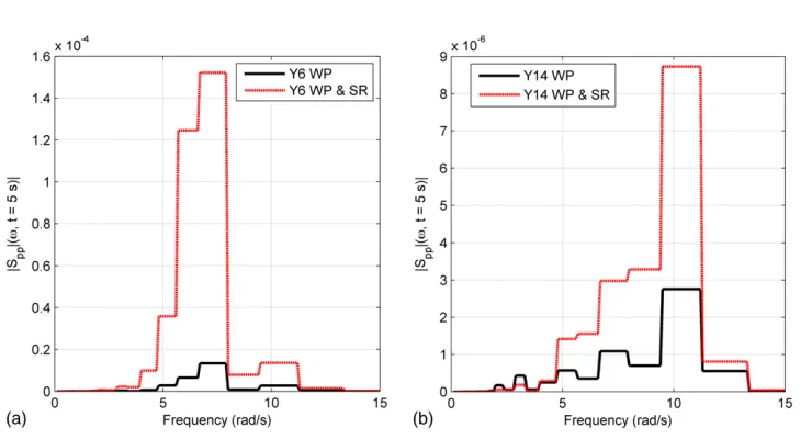
respec-533 tively. Figs.10(a and b)show the corresponding PSDs att55 s.

534 The effects of site-response on the amplitude nonstationarity and on

535 reducing the rate of decay of the RMS response envelope values in

536 time, as seen in Fig.6(b), are also observed in Figs.8(b)and9(b).

537 Figs.10(a and b)show that compared with the case with only the

538 wave-passage effect considered, the frequency content exhibits

539 stronger nonstationary and the peaks of the instantaneous PSDs are

540 higher in the case of combined wave-passage and site-response

541 effects. In addition, the attenuation of the response energy is slower

542 in time. Similar trends are observed in the EPSD of the column

Table 2. Estimated

11 Parameters for Kanai-Tajimi Frequency Response Function

Soil column vsðrad=sÞ zs(%) R-square RMSE

1 3.218 0.334 0.525 1.966

2 5.113 0.370 0.601 1.885

3 3.202 0.320 0.601 1.661

4 4.765 0.362 0.597 1.790

Note: R-square 5 coefficient of determination for RMSE; vs 5 soil characteristic frequency for Kanai-Tajimi;zs5damping ratio for Kanai-Tajimi.

Table 3.Estimated

12 Parameters for Clough-Penzien FRF

Soil column vsðrad=sÞ zs(%) vfðrad=sÞ zf(%) R-square RMSE

1 3.422 0.350 0.390 0.220 0.632 1.408

2 5.370 0.375 0.588 0.254 0.657 1.311

3 3.278 0.323 0.344 0.140 0.601 1.532

4 4.997 0.389 0.517 0.211 0.633 1.408

Note:R-square5coefficient of determination for RMSE;zf 5damping frequency for Clough-Penzien;zs5damping ratio for Kanai-Tajimi;vf 5soil characteristic frequency for Clough-Penzien;vs5soil characteristic frequency for Kanai-Tajimi.

543 _{relative horizontal displacements in Fig.11and the PSDs att55 s} 544 _{in Fig.12.}

545 _Conclusions

546 _{A wavelet-based evolutionary response formulation of multispan} 547 _{structures supported on a soil medium and subjected to spatially}

548 varying differential support motions including wave-passage and

549 site-response effects has been proposed in this paper. The

spatial-550 variability of support motions is formulated by bedrock parametric

551 coherency models, the time-lags from wave-passage effects, and

552 a proposed alternate way to represent site-response effect by

553 frequency-dependent time-lags. The earthquake energy content is

554 properly characterized by a composite PSDF constituted of parametric

Fig. 5.Variation of frequency-dependent time lags between the left support and other supports from site-response effects: (a) parametric Kanai-Tajimi FRF; (b) parametric Clough-Penzien FRF

Fig. 6.RMS value of relative vertical displacement: (a) at the midpoint of the left span (Y6); (b) at the midpoint of the midspan (Y14)

Fig. 8.PSD of relative vertical displacement at midpoint of left span using parametric Clough-Penzien (C-P) frequency response function: (a) wave-passage effect; (b) wave-wave-passage and site-response effects

Fig. 9.PSD of relative vertical displacement at midpoint of midspan using parametric Clough-Penzien (C-P) frequency response function: (a) wave-passage effect; (b) wave-wave-passage and site-response effects

555 _{surface-to-bedrock FRF and the bedrock power spectrum. The} site-556 _{compatible parametric FRFs are proposed to be characterized in this} 557 _{paper by carrying out a FEA of soil media beneath the supports.} 558 _{In an illustrative case study, a three-span, 2D hangar frame is} 559 _{analyzed using the proposed formulations. The time-lags stemming} 560 _{from the site-response effect, and computed from different FRFs,} 561 _{show different variations in trend. The site-response effect adds} 562 _{frequency nonstationarity to the frame responses and results in an} 563 _{increase of such responses with slower attenuation in time.} 564 _{This paper proposes a more accurate seismic analysis of} long-565 _{span multisupport structures because it accounts for the} non-566 _{stationarities in both amplitude and frequency of excitations and} 567 _{properties and variation of soil media beneath the supports; it offers} 568 _{a more realistic representation of earthquake energy content. The} 569 _{proposed formulations are generally applicable for any} wavelet-570 _{based functions and structures.}

571 _{Acknowledgments}

572 _{This research is partially funded under the EU FP7 Marie Curie} 573 _{IAPP project NOTES (grant No. PIAP-GA- 2008-230663). The}

574 authors are grateful for the support. The authors also thank the

anon-575 ymous reviewers who have given valuable comments.

576 References

577 Basu, B., and Gupta, V. K. (1997).“Non-stationary seismic response of

578 MDOF systems by wavelet modelling of non-stationary processes.”

579

Earthquake Eng. Struct. Dynam., 26(12), 1243–1258.

580 Basu, B., and Gupta, V. K. (1998).“Seismic response of SDOF system by

581 wavelet modeling of non-stationary processes.”J. Eng. Mech., 10.1061/

582 (ASCE)0733-9399(1998)124:10(1142), 1142–1150.

583 Basu, B., and Gupta, V. K. (2000).“Stochastic seismic response of SDOF

584 systems through wavelets.”Eng. Struct., 22(12), 1714–1722.

585 Boore, D. M. (2003).“Simulation of ground motion using the stochastic

586 method.”Pure Appl. Geophys., 160(3–4), 635–676.

587 Brinkgreve, R. B. J., Broere, D., and Waterman, D. (2008).PLAXIS 2D

588 version 9.0 manual, PLAXIS, Delft, Netherlands.

589 Chakraborty, A., and Basu, B. (2008).“Nonstationary response analysis of

590 long span bridges under spatially varying differential support motions

591 using continuous wavelet transform.”J. Eng. Mech., 10.1061/(ASCE)

592 0733-9399(2008)134:2(155), 155–162.

593 Clough, R. W., and Penzien, J. (2003).Dynamics of structures, McGraw

594 Hill, New York.

Fig. 11.PSD of relative horizontal displacements at the top offirst column using parametric Clough-Penzien (C-P) frequency response function: (a) wave-passage effect; (b) wave-passage and site-response effects

595 Deodatis, G. (1996).“Non-stationary stochastic vector processes: Seismic 596 ground motion applications.”Probab. Eng. Mech., 11(3), 149–168. 597 der Kiureghian, A. (1996).“A coherency model for spatially varying ground 598 motions.”Earthquake Eng. Struct. Dynam., 25(1), 99–111.

599₈ Dinh, N. V., and Basu, B. (2012).“Zero-pad effects on conditional simu-600 lation and application of spatially-varying earthquake motions.”Proc., 601 6th European Workshop on Structural Health Monitoring, Æwww 602 .ewshm2012.com/Portals/98/BB/tu3d3.pdfæ.

603 Dumanogluid, A. A., and Soyluk, K. (2003).“A stochastic analysis of long 604 span structures subjected to spatially varying ground motions including 605 the site-response effect.”Eng. Struct., 25(10), 1301–1310.

606 Gurley, K., and Kareem, A. (1999).“Application of wavelet transforms 607 in earthquake, wind, and ocean engineering.”Eng. Struct., 21(2), 608 149–167.

609 Hao, H. (1994).“Ground-motion spatial variation effects on circular arch 610 responses.”J. Eng. Mech., 10.1061/(ASCE)0733-9399(1994)120:11(2326), 611 2326–2341.

612 Hao, H., Olivera, C. S., and Penzien, J. (1989).“Multiple-station ground 613 motion processing and simulation based on SMART-I array data.”Nucl.

614 Eng. Des., 111(3), 293–310.

615 Harichandran, R. S., and Vanmarcke, E. H. (1986).“Stochastic variation of 616 earthquake ground motion in space and time.”J. Eng. Mech., 10.1061/

617 (ASCE)0733-9399(1986)112:2(154), 154–174.

618 Iyama, J., and Kuwamura, H. (1999).“Applications of wavelets to analysis 619 and simulation of earthquake records.”Earthquake Eng. Struct. Dynam.,

620 28(3), 255–272.

621 Kijewski-Correa, T., and Kareem, A. (2006). “Efficacy of Hilbert and 622 wavelet transforms for time-frequency analysis.”J. Eng. Mech., 10.1061/ 623 (ASCE)0733-9399(2006)132:10(1037), 1037–1049.

624 Konakli, K., and der Kiureghian, A. (2012).“Simulation of spatially varying 625 ground motions including incoherence, wave-passage and site-response 626 effects.”Earthquake Eng. Struct. Dynam., 41(3), 495–513.

627 Kramer, S. L. (1996).Geotechnical earthquake engineering, Prentice Hall, 628 Upper Saddle River, NJ.

629 Loh, C. H., and Ku, B. D. (1995).“An efficient analysis of structural response

630 for multiple-support seismic excitations.”Eng. Struct., 17(1), 15–26.

631 Luco, J. E., and Wong, H. L. (1986).“Response of a rigid foundation to

632 a spatially random ground motion.”Earthquake Eng. Struct. Dynam.,

633 14(6), 891–908.

634 MATLAB[Computer software]. Natick, MA, MathWorks. ₉

635 Priestley, M. B. (1981).Spectral analysis and time series, Academic Press,

636 New York.

637 Shinozuka, M., and Sato, Y. (1967).“Simulation of nonstationary random

638 processes.”J. Eng. Mech. Div., 93(1), 11–40.

639 Spanos, P. D., and Failla, G. (2004).“Evolutionary spectra estimation using

640 wavelets.”J. Eng. Mech., 10.1061/(ASCE)0733-9399(2004)130:8(952),

641 952–960.

642 Spanos, P. D., and Kougioumtzoglou, I. A. (2012).“Harmonic wavelets

643 based statistical linearization for response evolutionary power spectrum

644 determination.”Probab. Eng. Mech., 27(1), 57–68.

645 Spanos, P. D., Tezcan, J., and Tratskas, P. (2005).“Stochastic processes

646 evolutionary spectrum estimation via harmonic wavelets.” Comput.

647

Methods Appl. Mech. Eng., 194(12–16), 1367–1383.

648 Tratskas, P., and Spanos, P. D. (2003).“Linear multi-degree-of-freedom

649 system stochastic response by using the harmonic wavelet transform.”

650

J. Appl. Mech. 70(5), 724–731.

651 Trifunac, M. D., and Brady, A. G. (1975).“A study on the duration of strong

652 earthquake ground motion.”Bull. Seismol. Soc. Am., 65(3), 581–626.

653 Zerva, A. (2009).Spatial variation of seismic ground motions: Modeling

654 and engineering applications, Taylor & Francis, Boca Raton, FL.

655 Zerva, A., and Zervas, V. (2002). “Spatial variation of seismic ground

656 motions: An overview.”Appl. Mech. Rev., 55(3), 271–297.

657 Zhang, Y. H., Li, Q. S., Lin, J. H., and Williams, F. W. (2009).“Random

658 vibration analysis of long-span structures subjected to spatially varying

659 ground motions.”Soil. Dyn. Earthquake Eng., 29(4), 620–629.

660 Zhou, Z., and Adeli, H. (2003). “Time-frequency signal analysis of

661 earthquake records using Mexican hat wavelets.”Comput. Aided Civ.

662

Q:1_Please check that ASCE Membership Grades (Member ASCE, Fellow ASCE, etc.) are provided for all authors who are members.

Q:2_Please give a specific reference for ‘‘Kanai-Tajimi’’.

Q:3_Please give a specific reference for ‘‘Clough-Penzien’’.

Q:4_The numbered sections and subsections were styled to journal requirements in this paragraph and the one following. Please read the changes carefully and the rewording done to make the paragraph address the sections and subsections in a consistent manner. Kindly check and confirm or amend these changes.

Q:5_AU: What does ‘‘dyn’’ stand for? Please convert to SI units.

Q:6_Please give a reference for ‘‘Duhamel’s integral’’.

Q:7_Please spell out ‘‘EPSD’’ here, at first mention.

Q:8_Please give a date of access for ‘‘Dinh and Basu 2012.’’

Q:9_Please provide version number for MATLAB.

Q:10_For Table 1, please check and confirm or amend the defined terms. Please also give a definition for ‘‘E’’ and ‘‘v’’.

Q:11_For Table 2, please check and confirm or amend the defined terms.

Q:12_For Table 3, please check and confirm or amend the defined terms.

AUTHOR QUERIES