Concrete Analysis and Trade-Offs for the (Complete Tree) Layered Subset
Difference Broadcast Encryption Scheme
Sanjay Bhattacherjee and Palash Sarkar Applied Statistics Unit
Indian Statistical Institute
203, B.T.Road, Kolkata, India - 700108.
[email protected] and [email protected]
Abstract
Two key parameters of broadcast encryption (BE) schemes are the transmission size and the user storage. Naor-Naor-Lotspiech (2001) introduced the subset difference (SD) scheme achieving a good trade-off between these two parameters. Halevy-Shamir (2002) introduced the idea of layering to reduce user storage of the NNL scheme at the cost of increased transmission overhead. Here, we introduce several simple ideas to obtain new layering strategies with different trade-offs between user storage and transmission overhead. We define the notion of storage minimal layering and describe a dynamic programming algorithm to compute layering schemes for which the user storage is the minimum attainable using layerings. Further, the constrained minimization problem is considered. A method is described which yields BE schemes whose transmission overhead is not much more than the SD scheme but, whose user storage is still significantly lower.
Finally, anO(rlog2n) algorithm is obtained to compute the average transmission overhead for any layering based scheme wherer out ofnusers are revoked. This algorithm works for any layering strategy and also for arbitrary number of users. The algorithm has been used here to generate all data for the average transmission overhead.
Keywords: Broadcast encryption; subset difference; layering; transmission overhead; user storage
1
Introduction
Digital rights management systems like Pay-TV and content protection in HD-DVD and Blu-Ray discs can be modelled as follows. There is a set of users and a centre which broadcasts messages. For each message, the centre decides on a set of privileged users which should be able to access the message while the other users (revoked) should not be able to do so. A cryptographic system achieving such a functionality is called a broadcast encryption scheme [1, 2].
Naor, Naor and Lotspiech (NNL) [3] introduced an important BE scheme called the subset difference (SD) method. This scheme has been adopted as a standard for content protection in HD-DVD and Blu-ray discs [4]. The NNL-SD scheme is defined for nusers where n is a power of two, i.e.,n = 2`0 for some `0 ≥0. The users
are considered to be the leaves of a full binary tree having `0 levels. Each user needs to store `0(`0+ 1)/2 k-bit
strings where kis the key length of the underlying symmetric key cryptosystem. Ifr users are revoked, then the worst case header length (i.e., the number of encryptions of the session key) is 2r−1 [3], while the average case header length turns out to be at most 1.25r for practical situations (see [5] for a detailed analysis). The header length and the user storage for the SD scheme have been discussed in details in Section 2. The trade-off between user storage and average header length turns out to be very well suited for real-life applications. Further, the scheme itself is quite elegant and reasonably easy to implement.
A later work by Halevy and Shamir [6] introduced a variant of the SD method called the layered subset difference (LSD) scheme. The basic idea is to partition the tree into several layers which gives the name of the scheme. A different trade-off is obtained. User storage is reduced in the LSD method to`30/2 but, the maximum possible header length grows to 4r−3. In [6], based on simulation results, it is remarked that the average header length is around 2r. Compared to the SD method, the LSD method reduces the user storage at the cost of increasing the header length.
1.1 Our Contributions
We work within the ambit of the NNL-SD scheme [3] and the idea of layering introduced in [6]. The Halevy-Shamir (HS) layering works for n= 2`0 users where `
0 is a perfect square. This limits its usage to very specific
number of users (24,29,216,225). Two natural extensions of the HS layering strategy that work for values of` 0
that may not be a perfect square (and hence subsume the HS layering strategy) are considered. While both have the same storage requirement, one of them is experimentally seen to have lower average header length. We call this the extended HS or e-HS layering.
The first problem that we tackle is whether the user storage can be lowered further than the e-HS layering strategy. To this end, we introduce the notion of storage minimal layering. For such a strategy, the user storage requirement is the minimum possible that can be obtained from 2-way splitting of SD subsets using layerings. An
O(`3
0) time andO(`20) space dynamic programming algorithm is presented to compute storage minimal layerings.
In the HS layering strategy, the root node of the user tree is treated as a special level. We show that removing this condition yields a scheme where the user storage is significantly reduced while the effect on the average header length is negligible. The resulting storage minimal schemes result in user storages which are between 18% to 24% lower than that required by the (extended) Halevy-Shamir layering scheme. We note that our work does not provide any asymptotic improvement in user storage compared to the Halevy-Shamir scheme. Rather, our work provides concrete improvement in user storage for all practical values of n and also an algorithm to compute the corresponding layering strategies.
Simply minimizing user storage is only one aspect of the problem. We consider the constrained minimization problem whereby one tries to minimize the user storage but, without increasing the actual values of the average header length significantly beyond that achieved by the SD scheme. This is a difficult problem to solve analyti-cally. Instead, we show how to tackle the problem empirianalyti-cally. Given some idea about the number of users that would be revoked, we show how one may use this information to design a layering strategy for which the average header length is almost as small as the SD scheme. The user storage for such a layering scheme is significantly less than that of the SD scheme. Concrete practical examples are provided and it is shown how to tackle this problem for any practical value of the number of users.
the average header length. In this approach, for a fixed n and r, a set of r users are randomly revoked and the cover generation algorithm is applied to compute the corresponding header length. This process is repeated many times and the average of the different header lengths is taken to be an estimate of the actual value of the expected header length. Each run will require O(n) space (and hence alsoO(n) time) to compute the cover and hence the header length. In contrast, our algorithm does away with the need of performing such a simulation study. Given n and r, it directly computes the expected header length when r out of n users are uniformly revoked. Since r will be much smaller than n for practical scenarios, our algorithm will be faster and require much lesser space. The algorithm is of interest in its own right as it will be a useful tool to practitioners who may wish to quickly calculate the average header length for different broadcast scenarios.
1.2 Previous and Related Works
Before [3] and [6], BE schemes using resilient functions and their analysis were proposed in [7, 8]. Subsequent to [3] and [6], there have been some follow-up work analyzing the average header lengths of the SD and LSD schemes. In [9], a generating function is obtained for counting the number of ways p users out of n can be given access privilege so that the header length will be h. For a given n and p, the generating function was used to obtain equations to compute the expected header length. The authors however mentioned that their equations were “complex to compute and difficult to gain insight from”. Consequently, they went forward to find approximationsfor the same. In [10], this analysis of the expected header length was continued and it was shown that the standard deviations are small compared to the expected values, as the number of users gets large. Combinatorial analysis of the worst case header length of the SD method has been done in [11]. Lower bounds on the header length of the SD and LSD schemes were found in [12]. All of these works considered the number of users to be a power of two. In [5], this condition was relaxed and the SD method was extended to the CTSD method. A detailed combinatorial and probabilistic analysis of the CTSD method was carried out.
Several works [13, 14] on the combinatorics behind broadcast encryption schemes and different generic bounds on the efficiency parameters have been done. In [15], a generic method for constructing BE schemes from pseudo-random generators was proposed. While NNL [3] and most follow-up works consider BE for stateless user devices, BE schemes for low-state devices were proposed in [16].
Several other BE schemes have been proposed. Linear algebraic techniques have been used in [17] to find a family of broadcast encryption schemes called linear broadcast encryption schemes. The same authors had also proposed key pre-distribution methods based on linear algebraic techniques in [18]. Another interesting work on BE is [19], that works on the idea of “one key per punctured interval”. In [19], the worst case header length has been brought down to r or below for the first time, but at the cost of increasing user storage. For n= 228 and r = 210, the header length is belowr at the cost of 3.4×10⁸ times the storage of the SD scheme. Moreover, the
method is more complicated than the SD scheme.
BE schemes have also been proposed in the public key setting. In a public-key based BE, anybody can broadcast to a group of users in the system. We do not consider public key BE in this work and instead refer the reader to relevant work such as [20, 21]. For this paper, by BE we will mean symmetric key BE.
2
Subset Cover Framework
Suppose there are n users. In the subset cover revocation framework, a collection S of subsets of {1, . . . , n} is defined in a manner such that any set S ∈ S has an associated key and any subset of {1, . . . , n} which is not in S does not have any key associated with it. For a user u, let Su ={S ∈ S : u ∈S}. User u is given secret information Iu such that it can construct the key associated with any set inSu.
j
i
Figure 1: The subset S(i)\ S(j) of users.
G_L (LABEL_i) G_L (G_L (LABEL_i))
G_R (G_L (G_L (LABEL_i))) LABEL_i
Figure 2: Key for S(i) \ S(j) is L
i,j = GM(GR(GL(GL(LABELi)))).
i
Special Level
j k
Figure 3: The subsetS(i)\ S(j) split intoS(i)\ S(k) and S(k)\ S(j).
LABEL_i
G_L (LABEL_k)
G_R (G_L (LABEL_k)) G_L (LABEL_i)
LABEL_k Special Level
Figure 4: Key for S(i) \ S(k) is L
i,k = GM(GL(LABELi)) and for S(k) \ S(j) is Lk,j = GM(GR(GL(LABELk))).
key and the session key is encrypted with the keys associated with the subsets in the cover. The encrypted message forms the body while the different encryptions of the session key forms the header. So, the number of subsets in the cover determine the header length of the broadcast. Loosely speaking, this number itself is called the header length of the transmission.
To decrypt, a user first determines to which subset of the cover it belongs. Then, using its secret information, it generates the key associated with this subset. Decrypting the appropriate component of the header with this key, the user obtains the session key and then decrypting with the session key the user obtains the actual message. Two parameters are of crucial interest. The size of the secret informationIu that is to be stored by a useru
and the average or expected length of a broadcast header. Basic intuition tells us that as the number of elements in S grows, it should be possible to cover a privileged setT with lesser number of elements and so the average header length will decrease. On the other hand, asS grows, the size of Su also grows and this should lead to an
increase in the size of Iu. Thus, the average header length and the user storage are two competing parameters.
2.1 The Subset Difference Scheme
The SD scheme introduces a major novelty in definingS such that there is a compact way of representingIu. In
the original SD scheme, the number of users n is a power of 2, say n= 2`0. Consider the users to be the leaves
of a full binary tree. Each node in the tree represents the users at the leaf level of the tree rooted at that node. Suppose iis a node of the tree and let S(i) denote the leaves of the subtree rooted at i. Let j be a node in the
subtree rooted ati. Then for the SD scheme, the set S consists of the subsets S(i)\ S(j) for all possible choices
of node iand all possible nodes j 6=iin the subtree rooted at ias shown in Figure 1. These subsets are called SD subsets.
A clever algorithm is used to define the key associated with an SD subset S(i)\ S(j). First each node i in
pseudo-random generator (PRG) G:{0,1}k→ {0,1}3k is used. Let G(seed) be written as the concatenation of 3k-bit
strings GL(seed), GM(seed) and GR(seed). Suppose that a node j in the subtree rooted at node i is reached
from node i by the moves ‘left’, ‘left’ and ‘right’. Then the label of j derived from LABELi is LABELi,j = GR(GL(GL(LABELi))) and the key associated with the setS(i)\ S(j) isLi,j =GM(GR(GL(GL(LABELi)))) as
shown in Figure 2. This easily extends to any appropriate pair of nodesiandj. The stringLi,j is a k-bit string
and the value of k is determined by the key size of the underlying encryption algorithm.
Recall that users are at the leaf level of the tree. The leaf level is numbered 0 and level numbers increase up to `0 which is the level number of the root. For any user u, the user storage Iu is defined in the following
manner. Consider the path from the node u to the root and let i be a node on this path at level` > 0 of the tree. Let i1, . . . , i` be the siblings of the nodes on the path from u toi(including u but not including i). Then
for each suchi, useru gets the labelsLABELi,i1, LABELi,i2, . . . , LABELi,i`. The value of `varies from 0 to`0 and so each user gets`0(`0+ 1)/2 labels. The total size ofIu isk`0(`0+ 1)/2 bits where kis the size of the seed
of the PRG. Since k is fixed, it is enough to consider only the number of labels as determining the size of user storage.
The labels provided to a user are sufficient for the user to construct the key corresponding to any element in
Su. To see this suppose thatiis a node on the path fromu to the root and j is a node in the subtree rooted at
i such that u ∈ S(i)\ S(j). Since u is not in S(j) and both u and j are in the subtree rooted at i, the paths to
root from these two nodes intersect for the first time at some nodevwhich is also in the subtree rooted ati. Let
v1 be the first node in the path fromv toj. Thenv1 is the sibling of some nodev2 in the path fromu toiand
so u hasLABELi,v1. From this label, u can generate LABELi,j by applying GL and GR appropriately and so
can generateLi,j =GM(LABELi,j). ThisLi,j is the key corresponding to the setS(i)\ S(j). So,u can generate
keys for any subset inSu.
It is also required to argue that u cannot generate keys for any other subset in S. In the SD scheme, any subset in S is of the form S(i)\ S(j). If u is not in such a subset, then u is either not in S(i) or it is in S(j).
In either case, it is not too difficult to see that u does not obtain information which allows it to generate Li,j.
See [3] for more details.
2.2 The Layered Subset Difference Scheme
The point of the LSD scheme is to reduce the user storage in the SD scheme at the cost of increasing the header length. Reduction in the user storage is achieved by reducing the size of S. As in the SD scheme, the LSD scheme also considers the number of users to be of the form 2`0 where the users form the leaves of a full binary
tree. The major difference between the SD and the LSD schemes is that in the LSD scheme the levels of the tree are partitioned into layers. Some of the levels are marked as“special”. The collection of levels between (and including) two consecutive special levels is called a layer. The levels are numbered with the bottom-most level having the number 0, increasing to the top. The length of a layer is the difference between the numbers of the special levels enclosing the layer.
2.2.1 The Halevy-Shamir Layering Strategy
The layering strategy described in [6] is as follows:
“The root is considered to be at a special level, and in addition we consider every level of depth
k·p
log (n) for k= 1. . .log (n) as special (wlog, we assume that these numbers are integers).”
We call this the Halevy-Shamir (HS) layering strategy. It assumes √`0(= √logn) to be an integer and hence `0 to be a perfect square. The “wlog” in the above statement is valid when one is interested in asymptotic analysis. For concrete values of n, the paper does not describe how to choose a layering scheme. This restricts the use of the scheme to very limited values ofn(of the form 2`0 where`
authors of [6] consider the case of n= 228 users and suggest a layering strategy with layers of size 6,6,6,5 and
5. However, they do not give any general description of how to choose the layer lengths when`0 is not a perfect square. We take up this issue later.
As a consequence of layering, an SD subset S(i) \ S(j) is defined to be in S if either of the following two
conditions hold:
• node iis at a special level;
• or, nodeiis not at a special level but, node j is in the same layer as level i.
This reduces the size of S and consequently ofSu. As a result, the size ofIu also reduces as we explain below.
The distribution of labels is done as follows. Suppose thatu is a user (i.e., a leaf node) andiis a node at level `
in the path from uto the root and i1, . . . , i` are the siblings of the nodes in the path fromutoi. If`is a special
level, then u is given LABELi,i1, . . . , LABELi,i` as in the SD scheme. Suppose ` is not a special level. Let`
0
be the first special level below iand consider the segment of the path from u toi which lies between `0 and `.
Supposeim, . . . , i` are the siblings of the nodes on this segment. Thenu gets LABELi,im, . . . , LABELi,i`. The net effect is that if iis not at a special level, it generates labels only up to the next special level (and not up to the bottom-most level). This leads to the reduction in the user storage.
The reduction in user storage is achieved at the cost of an increase in the header length. Suppose iis not at a special level and j is in the sub-tree rooted at i but not in the same layer as i. The SD scheme would associate the set S(i)\ S(j) to such an (i, j) pair. In the LSD scheme, this set is not present. Instead, the header
computation algorithm will cover this set in the following manner. Letk be the node in the first special level as one moves down the path from i to j. The sets S(i)\ S(k) and S(k)\ S(j) are both present in the LSD scheme
and it is easy to see that
S(i)\ S(j)=S(i)\ S(k) [ S(k)\ S(j).
This can be viewed as a two-way split of the set S(i)\ S(j). Figure 3 shows the splitting of the subsetS(i)\ S(j)
of Figure 1. The key assignment to the subsets in Figure 3 is shown in Figure 4. The work [6] also consider the possibility of multi-way split. But, the authors conclude that this leads to further reduction in user storage only for impractical values of the number of users. In this paper, we will not consider multi-way split.
As mentioned earlier, [6] does not mention how to generate a layering strategy when`0is not a perfect square. Later in Sections 3(3.1) and 3(3.2) below we look at two natural extensions of the HS layering strategy that can be adopted for 2`0 users for values of `
0 which may not be perfect squares.
3
General Layering Strategy
In general, a layering strategy`is denoted by the numbers of the special levels`0> `1> ... > `e−1> `e= 0. Let `= (`0, . . . , `e). The layering strategy has (e+ 1) special levels. It is sometimes more convenient to use another
formulation to denote the layering. For 1≤ i≤e, define di =`i−1−`i so thatdi’s are positive integers whose
sum is `0. Conversely, given any sequence of positive integersd= (d1, . . . , de) whose sum is `0, it is possible to
define a layering scheme where `i=`0−Pij=1dj.
The user storage for any such layering strategy `in general can be calculated as follows. Corresponding to each special level `i, a user has to store `i labels. Now consider the nodes in the layer bordered by `i and `i+1.
Corresponding to any non-special level j in this layer a user has to storej−`i+1 labels. So, the total number
following formula.
storage0(`) =
e−1
X
i=0 `i+
e−1
X
i=0 `i−1
X
j=`i+1+1
(j−`i+1)
=
e−1
X
i=0 `i+
e−1
X
i=0
`i−`i+1−1 X
j=1 j
=
e−1
X
i=0 `i+
1 2
e−1
X
i=0
(`i−`i+1)(`i−`i+1−1). (1)
A recursive description can be obtained as follows.
storage0(`0, `1, . . . , `e)
=`0+`1+· · ·+`e+
(`0−`1)(`0−`1−1) 2
+(`1−`2)(`1−`2−1) 2
+· · ·+(`e−1−`e)(`e−1−`e−1) 2
=`0+
(`0−`1)(`0−`1−1)
2 +storage0(`1, . . . , `e). (2) Equation (1) can be formulated in terms of the layer lengths d= (d1, . . . , de) as follows.
storage0(`) = `0(e+ 1)− e
X
i=1
(e−i+ 1)di
+1 2
e
X
i=1
di(di−1). (3)
If all the di’s are equal to d and `0 = e×d, then storage0(`) is given by `0(e+d)/2. This shows that the
user storage using e layers of length d each is the same as the user storage using d layers of length eeach. If all the layer lengths are equal, then the problem of minimizing the user storage is that of minimizing the sum
e+d subject to the constraint ed = `0. From this it is easy to see that the minimum value is attained for
e=d=√`0 and the corresponding value of user storage is` 3/2
0 . This justifies the choice made in [6]. Note that
the minimization here is in the context of all the layer lengths being equal.
It is easy to note that the layering strategy with each di = 1 or with e= 1 results in the SD scheme. The
supplementary material provides some further combinatorial results on general layering strategies.
3.1 The HS Layering with residual bottom layer
Let `0 be any positive integer and d≤`0. We write `0 =d(e−1) +p where 1≤p ≤d. Then the special levels
are
`0,`0−d,`0−2d,. . .,`−d(e−1), 0.
So, the tree will have a total of e+ 1 special levels (including the root level `0 and the leaf level 0) and elayers
out of which e−1 layers are of length d each and the last layer is of length p. Note that the length p of the bottom-most layer can equal dwhich will lead to elayers each of length d. We find it convenient to always have level 0 (leaf level) as a special level as this does not have any effect on either the user storage or the header length. The Halevy-Shamir (HS) layering strategy is a special case where `0 is a perfect square with d= √`0
3.2 The e-HS Layering Strategy
We now consider a layering strategy where the layer lengths are balanced. Write `0 =d(e−1) +p= (e−d+ p)d+ (d−p)(d−1) and define d0 = (d, . . . , d
| {z }
e−d+p
, d−1, . . . , d−1
| {z }
d−p
). Let ` be the layering strategy with a residual
bottom layer and`0 be the balanced layering strategy. Then, one can show thatstorage0(`) =storage0(`0). (The proof is given in the supplementary material.) So there is no difference between these two strategies in terms of user storage. Experimental results show that the average header lengths for both strategies are similar with that corresponding to the balanced strategy being slightly smaller. As an example, for `0 = 18,d0 = (5,5,4,4)
yields lesser expected header lengths thand= (5,5,5,3) for all r between 256 and 16384 while the user storage 75 is the same for both. We call the balanced strategy to be the extended HS or e-HS layering strategy. This strategy coincides with the layering scheme given in [6] forn= 28.
Using (3), it can be verified that storage requirement isO(log3/2n) for both the e-HS and the residual bottom layer strategies.
3.3 Root at a non-special level
In the HS layering [6] as well as its extensions given in Section 3(3.1) and Section 3(3.2), the root level `0 is
always taken as a special level. It is possible to obtain further reduction in user storage if we allow the root level to be a non-special level. Having the root as a special level contributes`0 labels to the user storage. If instead the root level is made non-special, then its contribution to the user storage will be `0−`1 labels. Given a sequence
of level numbers `, let storage1(`) be the number of labels required to be stored when the root (top-most) level is not special (and so, `1 is the first special level). Then the following relation holds.
storage1(`) = storage0(`)−`1. (4)
Combining this with (2) we get the following relation.
storage1(`0, . . . , `e) =
(`0−`1)(`0−`1+ 1) 2
+storage0(`1, . . . , `e). (5)
So, not having the root at a special level reduces the storage requirement by `1 labels. This can be quite significant. Consider the e-HS layering strategy where `0 =d×e and so`= (`0, `1, . . . , `e) where `i−`i+1 =d
for 0≤i < e. In this case, storage0(`) =`30/2 and storage1(`) =`30/2−(`0−` 1/2 0 ).
It is important to understand the effect on the header length when the root level is not special. During the computation of the cover, suppose that the root generates an SD subset, i.e., the SD cover finding algorithm returns a subset of the form S(0)\ S(j). Since the root is not at a special level, this subset may be split into two
ifj is not in the first layer. We argue that for reasonable values ofr (the number of revoked users), this effect is negligible. In fact, the argument is that the probability of the root generating an SD subset itself is small.
The root generates an SD subset only if exactly one of the two subtrees of the root node contains all the revoked users. Intuitively this probability is low even for moderate values of r. We provide some more justification. Suppose the revoked users are uniformly distributed, i.e.,r users are uniformly sampled one-by-one without replacement and revoked. Then the probability that the left subtree does not have any revoked user (and consequently the right subtree contains all of them) is
1−n/2
n 1− n/2
n−1
· · ·
1− n/2
n−r+ 1
=
1−1
2
1− 1
2 1− 1 n
!
· · · 1− 1
2 1−r−1 n
The probability that the right subtree does not have any revoked user is also equal to this value. So, the total probability that the header generates a subset is twice this value. For practical applications of BE, the number of users nwill be usually be much larger than the number of revoked usersr and so the ratio r/nwill be small. Then the above expression can be approximated by 2−r. This is negligible even for values of r as small as 20 or
so. Consequently, for practical situations, there will be almost no effect on the header length if the root level is not made special.
3.4 Storage Minimal Layering
For a given value of `0, let SML0(`0) denote a layering strategy ` (or equivalently is given by the sequence of
differences d), such that storage0(`) takes the minimum value among all possible layering strategies for a tree with `0 levels and having the root as a special level. Let #SML0(`0) denote storage0(`) where ` is a storage
minimal layering strategy. Similarly define SML1(`0) and #SML1(`0) that exclude the root level from being
special.
We describe a dynamic programming based algorithm to compute SML0(`0) (and subsequently SML1(`0)).
The idea of the algorithm is explained as follows. For a fixed value of`0, the number of layersecan vary from 1 to`0. The casese= 1 ande=`0 correspond to the SD scheme and in these two cases the user storage is known to be equal to `0(`0+ 1)/2. Let SML0(e, `0) denote a storage minimal layering using exactly e layers. Clearly,
the following relation holds.
#SML0(`0) = min 1≤e≤`0
#SML0(e, `0). (6)
Also,
#SML0(e, `0) = min (`0,...,`e)
storage0(`0, `1, . . . , `e) (7)
where the minimum is over all possible layering strategies (`0, `1, . . . , `e). Using (2)
#SML0(e, `0) =
min
1≤`1<`0
`0+
(`0−`1)(`0−`1−1)
2 + #SML0(e−1, `1)
.
(8)
This relation is the basis for the algorithm. Let Tabbe an `0×`0 table such that Tab[e][`0] = #SML0(e, `0). A
simpleO(`3
0) time dynamic programming algorithm can fill up this table as given in Algorithm 1.
Using (6) provides #SML0(`0) as the minimum value in column number `0 of Tab. Note that the minimum
may occur for more than one possible value of e. These values of `1 are reported during the computation. Let Λ(e, `0) be the list of all possible values of`1for which (8) holds. The above method can be extended to generate all possible layering strategies for which user storage is minimized.
An SML0 layering strategy ` can be generated as follows. Start with ` as the list containing only `0 and
keep on appending in the following manner to obtain the complete sequence. Letebe one of the possibilities for which Tab[e][`0] takes the minimum value; choose `1 as any one value from Λ(e, `0) and append to `; choose`2
as any one value from Λ(e−1, `1) and append to`; continue until 0 is appended to the list. All SML0 strategies
ALGORITHM 1: Dynamic Programming Algorithm to find Tab
Input: `0.
Output: An`0×`0 table TabwhereTab[e][`] contains the value of #SML0(e, `).
for`= 1 to`0 do
Tab[1][`] =Tab[`][`] =`(`+ 1)/2; end
for`= 2 to`0 do
fore= 2 to `−1 do
Tab[e][`] = min
1≤`1<`
`+(`−`1)(`−`1−1)
2 +Tab[e−1][`1]
end end
OnceTab is prepared, computing #SML1(`0) using (5) is easy.
#SML1(`0)
= min
e min`1
#SML0(e−1, `1) +
(`0−`1)(`0−`1+ 1)
2
= min
e min`1
Tab[e−1][`1] +
(`0−`1)(`0−`1+ 1)
2
. (9)
The first minimization is over the number of layers and the second minimization is over the value of the first special level. The possible corresponding layering strategies can also be easily recovered. It is to be noted that the SML1(`0) layerings are due to the minimization of the user storage by assuming the root to be at a non-special
level. It can be seen from (8) and (9) that in an SML0(`0) layering, if the root is made non-special, it might not
[image:10.595.175.439.301.369.2]necessarily result in an SML1(`0) layering and vice versa.
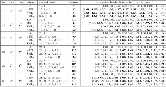
Table 1 shows values of user storage for SML strategies for some`0. For comparison, we also show the storage requirements for the SD scheme and the e-HS layering strategy. Compared to the SD scheme, the e-HS layering strategy reduces the storage requirement very significantly (both asymptotically as well as in practical numbers). Compared to the e-HS scheme the value of #SML0(`0) is slightly smaller and the value of #SML1(`0) is about
18% to 24% lower for the newly suggested values of`. So, given a value of `0, if the requirement is to minimize
the user storage, then the SML strategies offer better alternatives. They also guarantee that using 2-way splitting of SD subsets with layering, further lowering of storage cannot be achieved.
The effect of SML0(`0) and SML1(`0) strategies on the average header length is also shown in Table 1. For
computing the average header lengths, we have considered ten values ofr equally spaced betweenrmin andrmax.
The reported values are the average header lengths of the different schemes normalized by the average header length of the SD scheme. As an example, the first value 1.69 corresponding to the row for e-HS and `0 = 28
means that withn= 228users out of whichr= 210are uniformly revoked, the average header length of the e-HS
layering strategy is 1.69 times that of the SD scheme. One may note the following points.
1. For a fixed`0, there may be more than one SML0(`0) (resp. SML1(`0)) strategy which achieves storage of
#SML0(`0) (resp. #SML1(`0)). Table 2 gives the number of SML strategies for several values of`0. For `0 = 12, Table 3 lists all possible SML0(`0) and SML1(`0) strategies for `0 = 12. There, however, need
`0 rmin rmax scheme special levels storage normalized header lengths for (rmin, . . . , rmax)
12 22 26
SD 12,0 78 (1.00,1.00,1.00,1.00,1.00,1.00,1.00,1.00,1.00,1.00)
e-HS 12,8,4,0 42 (1.69, 1.59, 1.56, 1.56, 1.57, 1.57, 1.57, 1.56, 1.55,1.53,1.52) SML0 12,8,5,3,1,0 40 (1.68, 1.57, 1.54, 1.54, 1.54, 1.55, 1.55, 1.54, 1.54,1.53,1.52)
SML1 8,5,3,1,0 32 (1.68, 1.57, 1.54, 1.54, 1.54, 1.55, 1.55, 1.54, 1.54,1.53,1.52)
16 23 28
SD 16,0 136 (1.00,1.00,1.00,1.00,1.00,1.00,1.00,1.00,1.00,1.00)
HS 16,12,8,4,0 64 (1.63,1.65, 1.66, 1.64, 1.62, 1.60, 1.58, 1.57, 1.57, 1.56) SML0 16,11,7,4,2,1,0 61 (1.69,1.60, 1.63,1.65,1.65,1.64,1.63,1.62,1.60,1.59)
SML1 12,8,5,3,1,0 50 (1.63,1.64, 1.65, 1.63, 1.60, 1.58, 1.57, 1.56, 1.55, 1.54)
20 24 210
SD 20,0 210 (1.00,1.00,1.00,1.00,1.00,1.00,1.00,1.00,1.00,1.00)
e-HS 20,15,10,5,0 90 (1.64,1.72,1.69,1.66,1.64, 1.62, 1.61, 1.61, 1.60, 1.60) SML0 20,15,10,6,3,1,0 85 (1.64,1.72,1.69,1.66,1.63, 1.62, 1.61, 1.60, 1.60, 1.60)
SML1 15,10,6,3,1,0 70 ((1.64,1.72,1.69,1.66,1.63, 1.62, 1.61, 1.60, 1.60, 1.60)
24 25 212
SD 24,0 300 (1.00,1.00,1.00,1.00,1.00,1.00,1.00,1.00,1.00,1.00)
e-HS 24,19,14,9,4,0 116 (1.62,1.64,1.62,1.64,1.67, 1.69, 1.71, 1.71, 1.72, 1.72) SML0 24,18,12,7,3,1,0 112 (1.65,1.74,1.70,1.67,1.65, 1.63, 1.63, 1.62, 1.62, 1.63)
SML1 18,12,8,5,3,1,0 94 (1.65,1.74,1.69,1.66,1.63, 1.62, 1.61, 1.60, 1.60, 1.60)
25 25 212
SD 24,0 325 (1.00,1.00,1.00,1.00,1.00,1.00,1.00,1.00,1.00,1.00)
HS 25,20,15,10,5,0 125 (1.62,1.64,1.62,1.64,1.67, 1.69, 1.71, 1.71, 1.72, 1.72) SML0 25,19,13,9,6,3,1,0 119 (1.65,1.74,1.69,1.66,1.63, 1.62, 1.61, 1.60, 1.60, 1.60)
SML1 19,13,9,6,3,1,0 100 (1.65,1.74,1.69,1.66,1.63, 1.62, 1.61, 1.60, 1.60, 1.60)
28 26 214
SD 28,0 406 (1.00,1.00,1.00,1.00,1.00,1.00,1.00,1.00,1.00,1.00)
e-HS 28,22,16,10,5,0 146 (1.64,1.65,1.63, 1.66, 1.69, 1.71, 1.73, 1.74, 1.75, 1.75) SML0 28,21,15,10,6,3,1,0 140 (1.65,1.70,1.65,1.63, 1.62, 1.63, 1.64, 1.66, 1.67, 1.68)
[image:11.595.30.569.129.411.2]SML1 22,16,11,7,4,2,0 119 (1.64,1.65,1.62, 1.64, 1.67, 1.69, 1.70, 1.71, 1.72, 1.72)
Table 1: Comparison of user storage and expected header lengths between e-HS LSD and SML. The tuples contain header lengths normalized with the SD header lengths corresponding to the values ofrin (rmin, . . . , rmax)
respectively.
`0 no. of SML0(`0) layerings no. of SML1(`0) layerings
12 10 10
16 6 15
20 6 1
24 35 35
25 35 21
[image:11.595.217.558.542.666.2]28 1 8
Table 2: The number of SML0(`0) and SML1(`0)
layer-ing strategies for various values of `0.
10 Special levels for SML0(12) 10 Special levels for SML1(12)
12,7,4,2,1,0 8,4,2,1,0
12,8,4,2,1,0 8,5,2,1,0
12,8,5,2,1,0 8,5,3,1,0
12,8,5,3,1,0 9,5,2,1,0
12,7,3,1,0 9,5,3,1,0
12,7,4,1,0 9,6,3,1,0
12,7,4,2,0 8,4,1,0
12,8,4,1,0 8,4,2,0
12,8,4,2,0 8,5,2,0
12,8,5,2,0 9,5,2,0
Table 3: List of SML0(`0) and SML1(`0) layering
2. For `0 = 32, Tab has been computed and reported in Table I of the supplementary material. It gives the
values of the minimum storage for every 1≤`0 ≤32 and 1≤e≤`0. For a particular`0 ande, it also gives the values of`1for which (8) holds. As an example, we see that for`0 = 32 ande= 8, #SML0(e, `0) = 172
and the values of `1 are 24 and 25. All possible SML0(`0) strategies for 1≤`0 ≤32 can be obtained from
this table and the SML1(`0) strategies can subsequently be found using (9).
3. As discussed earlier, if the root level is made non-special in an SML0 strategy, it may not lead to an SML1
strategy and vice versa. Table 3 shows that while the SML0 strategy `= (12,8,4,2,1,0) gives rise to an
SML1 strategy`= (8,4,2,1,0) by making the root level non-special, the SML0strategy`= (12,7,4,2,1,0)
does not. On the other hand, the SML1 strategy`= (9,5,2,1,0) is not generated from an SML0 strategy.
4. Extensive experimentation have shown that for practical values of r, there is no significant difference between the average header lengths of SML0 and SML1 strategies that differ at only the root being at a
special level or not. For `0 = 12 and 16, the reported SML0 strategy with the root level made non-special
turns out to be an SML1 strategy (as reported in Table 1) with minimum expected header lengths. This
supports the theoretical justification described before. However, for `0= 20, it turns out that making the
root level of the SML0 strategy non-special does not give rise to an SML1 strategy. For `0 = 24 and 28, it
is again true that making the root level of the reported SML0 strategy non-special gives rise to an SML1
strategy. But there are other SML1 strategies that further reduce the expected header lengths and hence
we report those strategies in Table 1.
5. In general, the header length of the e-HS scheme is smaller than that of SML0 and SML1. This is somewhat
expected, since user storage in SML is smaller. On the other hand, the user storage is not the only determining factor. The actual layering strategy also plays a role and in some cases it turns out that the average header length in SML turns out to be smaller than that in e-HS. We do not have an analytical justification for this. Intuitively, it appears that for the number of revoked users that have been considered, the SML assigns keys to SD subsets which are more probable to occur in the header. As a result, in such cases, we see thatbothuser storage and average header length are reduced. These are marked in bold and are particularly noticeable for`0 = 24 and`0 = 28. In the context of AACS standard [4], SML1 for`0 = 28
is of particular significance.
3.5 Constrained Minimization of User Storage
From the viewpoint of minimizing communication bandwidth it is of interest to minimize the average header length. This is minimized when the number of keys is maximized which happens for the SD scheme, i.e., when all the levels are considered to be special levels or there is only a single layer. Taking the average header length for the SD scheme as a benchmark, one may ask the question as to how much the user storage can be reduced from that required by the SD scheme without significantly increasing the corresponding values for the average header length? The expression for the average header length (as can be derived from (11), (13) and Proposition 2 given later) is rather complicated and it appears quite impossible to have an analytical solution to this question. Instead, we use our average header length computation program (developed in Section 4.3) to study this behaviour for concrete practical values of n,r and layering strategies`. It turns out that it is indeed possible to significantly reduce the user storage values with minimal increase in the average header length values. Our approach is the following. The increase in header length due to layering occurs because of the fact that certain SD subsets are split into two. If we can avoid making too many splits, then we can ensure that the header length does not increase by too much in comparison to the SD scheme. Consider an SD subset of the form S(i)\ S(j) where node iis at level`. We say that this subset is generated from the node i. Now, consider
strategy is to ensure that SD subsets originating from levels which contribute most to the header are not split. This mitigates the effect of splits.
Suppose there are n users and r of them are revoked. In [5] it has been shown that the probability that a particular node at level `generates a subset in the header is 2(ηr(n,2`−1)−ηr(n,2×2`−1)−ηr(n,3×2`−1) + ηr(n,4×2`−1)) whereηr(n, x) = (1−x/n)(1−x/(n−1))· · ·(1−x/(n−r+ 1)) ifn > r−1 else 0. Since there
are 2`0−` nodes at level `, the expected number of subsets arising from all nodes at level `is
2`0−`+1(ηr(n,2`−1)−ηr(n,2×2`−1)
−ηr(n,3×2`−1) +ηr(n,4×2`−1)). (10)
This expression gives the expected contribution of a level to the header size for a given r.
For a fixednandr, one can consider the problem of finding`for which (10) is maximized. Analytically, this seems to be very difficult to do. Instead we have done extensive experimentation. Empirical values suggest that the maximum occurs for some level `≤`0− blog2rc. Also, for` > `0− blog2rc, the value of (10) is quite small.
Based on this empirical evidence we suggest the following layering strategy.
• Make level`0− blog2rc special. Level 0 is also special.
• No level 0< ` < `0− blog2rc is made special. In terms of user storage and expected header length this is
equivalent to making all levels ` < `0− blog2rcto be special.
• The root level is not made special.
• At most one level that is midway between `0 and `0 − blog2rc is made special. While this does not significantly affect header size, it can reduce the storage requirement.
We call this the constrained minimization layering (CML) strategy. This strategy will ensure that if ` ≤ `0 − blog2rc, then no SD subset generated from level ` or below will be split. Splits will occur only for SD subsets originating from levels above `. But, the expected number of such subsets is small and so, splits will occur only for a small number of SD subsets.
One issue with this strategy is that the value ofr will not be known a priori while the layering scheme will have to be decided upon during the design phase itself. A way out is to make an assumption about the minimum number of revoked users that will occur in the steady state operation of the BE scheme. For example, in AACS with 228users one may assume that in the steady state at least 210users will be revoked due to equipment piracy
problems.
Suppose thatrmin is the minimum number of users that will be revoked during each broadcast. The above
layering strategy is used withrmin. Suppose now that during a broadcast, the number of usersr that is actually revoked is greater than rmin. Then from our empirical evidence the level for which the average header length is maximized will be `0− blog2rc. Since this value is less than`0− blog2rminc, none of the subsets generated from
this level will be split. So, the feature of not splitting a large number of SD subsets is still retained.
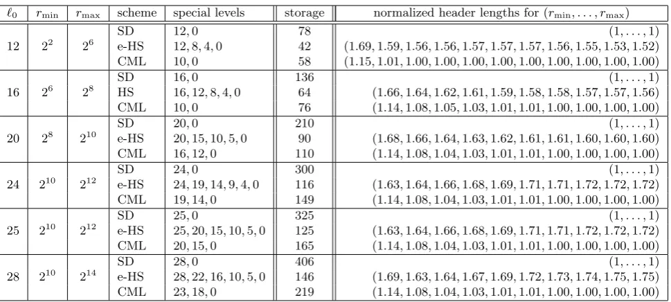
Table 4 shows a comparison between the SD scheme, the e-HS layering scheme and a constrained minimization layering scheme as described above, in terms of both their user storage requirement and the expected header length normalized with respect to the SD scheme. The average header length depends on the numberrof revoked users. So, for a given n= 2`0, we computed the expected header lengths for 10 equispaced values of r between
and including rmin and rmax. The values in the table illustrate the point that compared to the SD scheme, the
constrained minimization layering scheme substantially reduces the user storage with a small increase in the average header length.
The layering scheme is designed assuming that the number of revoked users is at leastrmin. What happens if
`0 rmin rmax scheme special levels storage normalized header lengths for (rmin, . . . , rmax)
12 22 26
SD 12,0 78 (1, . . . ,1)
e-HS 12,8,4,0 42 (1.69,1.59,1.56,1.56,1.57,1.57,1.57,1.56,1.55,1.53,1.52)
CML 10,0 58 (1.15,1.01,1.00,1.00,1.00,1.00,1.00,1.00,1.00,1.00,1.00)
16 26 28
SD 16,0 136 (1, . . . ,1)
HS 16,12,8,4,0 64 (1.66,1.64,1.62,1.61,1.59,1.58,1.58,1.57,1.57,1.56)
CML 10,0 76 (1.14,1.08,1.05,1.03,1.01,1.01,1.00,1.00,1.00,1.00)
20 28 210
SD 20,0 210 (1, . . . ,1)
e-HS 20,15,10,5,0 90 (1.68,1.66,1.64,1.63,1.62,1.61,1.61,1.60,1.60,1.60)
CML 16,12,0 110 (1.14,1.08,1.04,1.03,1.01,1.01,1.00,1.00,1.00,1.00)
24 210 212
SD 24,0 300 (1, . . . ,1)
e-HS 24,19,14,9,4,0 116 (1.63,1.64,1.66,1.68,1.69,1.71,1.71,1.72,1.72,1.72)
CML 19,14,0 149 (1.14,1.08,1.04,1.03,1.01,1.01,1.00,1.00,1.00,1.00)
25 210 212
SD 25,0 325 (1, . . . ,1)
e-HS 25,20,15,10,5,0 125 (1.63,1.64,1.66,1.68,1.69,1.71,1.71,1.72,1.72,1.72)
CML 20,15,0 165 (1.14,1.08,1.04,1.03,1.01,1.01,1.00,1.00,1.00,1.00)
28 210 214
SD 28,0 406 (1, . . . ,1)
e-HS 28,22,16,10,5,0 146 (1.69,1.63,1.64,1.67,1.69,1.72,1.73,1.74,1.75,1.75)
[image:14.595.57.542.87.305.2]CML 23,18,0 219 (1.14,1.08,1.04,1.03,1.01,1.01,1.00,1.00,1.00,1.00)
Table 4: Comparison of user storage and average header length for SD, e-HS LSD and the constrained minimiza-tion layering. The tuples contain header lengths normalized with the SD header lengths corresponding to the values of r in (rmin, . . . , rmax) respectively.
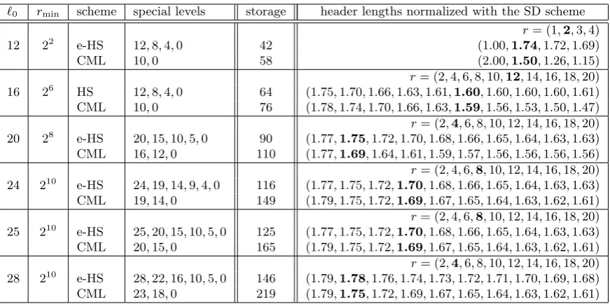
Table 5. Again the values of the average header length are normalized by that of the corresponding SD scheme. For comparison, we have also provided the average header lengths of the e-HS layering strategy. It is to be noted that the expected header lengths of the CML scheme are mostly better than the e-HS scheme. As an example, forn= 224, forr >6, the CML strategy gives smaller expected header lengths than the e-HS layering strategy.
Table 5 shows that for any value of n, the CML strategy leads to smaller expected header lengths for allr >15. To summarize, the constrained minimization layering strategy requires significantly lesser user storage than the SD scheme. In terms of the expected header length, it is as good as the SD scheme forr ≥rmin. Ifr < rmin, then it is better than e-HS layering but inferior to the SD scheme. It is to be noted that if r is small, then the absolute size of the header itself is not too large. As a result, the effective transmission overhead of the scheme will never be too high compared to the actual body of the message.
4
Header Length
The main point of the discussion in this section is to obtain an efficient algorithm for computing the expected header length for the layered SD schemes including the LSD scheme. The algorithm we obtain works for all possible values of the number of users. To ensure this, we first need to extend the scheme to handle arbitrary number of users. For the SD scheme, this was done in [5] by using the notion of complete binary trees. Here, we extend the scheme of [5] to handle layering as well.
4.1 Tackling Arbitrary Number of Users
In [3] and [6], the number of users has been taken to be a power of two, i.e.,n= 2`0. One has to consider dummy
users in the system to make the number of users a power of two. The inclusion of dummy users (considered revoked or privileged) increase the expected header length in the system. Hence, this is not always convenient as has been argued in details in [5].
`0 rmin scheme special levels storage header lengths normalized with the SD scheme
12 22
r= (1,2,3,4)
e-HS 12,8,4,0 42 (1.00,1.74,1.72,1.69)
CML 10,0 58 (2.00,1.50,1.26,1.15)
16 26
r= (2,4,6,8,10,12,14,16,18,20)
HS 12,8,4,0 64 (1.75,1.70,1.66,1.63,1.61,1.60,1.60,1.60,1.60,1.61)
CML 10,0 76 (1.78,1.74,1.70,1.66,1.63,1.59,1.56,1.53,1.50,1.47)
20 28
r= (2,4,6,8,10,12,14,16,18,20)
e-HS 20,15,10,5,0 90 (1.77,1.75,1.72,1.70,1.68,1.66,1.65,1.64,1.63,1.63)
CML 16,12,0 110 (1.77,1.69,1.64,1.61,1.59,1.57,1.56,1.56,1.56,1.56)
24 210
r= (2,4,6,8,10,12,14,16,18,20)
e-HS 24,19,14,9,4,0 116 (1.77,1.75,1.72,1.70,1.68,1.66,1.65,1.64,1.63,1.63)
CML 19,14,0 149 (1.79,1.75,1.72,1.69,1.67,1.65,1.64,1.63,1.62,1.61)
25 210
r= (2,4,6,8,10,12,14,16,18,20)
e-HS 25,20,15,10,5,0 125 (1.77,1.75,1.72,1.70,1.68,1.66,1.65,1.64,1.63,1.63)
CML 20,15,0 165 (1.79,1.75,1.72,1.69,1.67,1.65,1.64,1.63,1.62,1.61)
28 210
r= (2,4,6,8,10,12,14,16,18,20)
e-HS 28,22,16,10,5,0 146 (1.79,1.78,1.76,1.74,1.73,1.72,1.71,1.70,1.69,1.68)
[image:15.595.81.517.88.305.2]CML 23,18,0 219 (1.79,1.75,1.72,1.69,1.67,1.65,1.64,1.63,1.62,1.61)
Table 5: Comparison of average header length for r < rmin between e-HS layering strategy and the constrained minimization layering strategy.
the second last levels. The last level has all its nodes to the left side. An example of a complete subtree accommodating 13 users is shown in Figure 5. In this case`0 = 4 and choosing d= 2 gives two layers and three special levels as shown in the figure. When the number of users is a power of two, the corresponding tree is called a full binary tree. This difference in terminology between full and complete has been taken from the literature on data structures. We explain some terminology with respect to Figure 5. The left and the right subtrees of node 3 are the subtrees rooted at nodes 7 and 8 respectively. The sibling subtree of node 3 is the subtree rooted at node 4. The only non-full subtrees are those rooted at nodes 0, 2 and 5. We call the path labelled by the nodes 0, 2 and 5 to be the dividing path.
In general given n with 2`0−1 < n ≤2`0, it is possible to accommodaten users as the leaves of a complete
binary tree withnleaves. The root node is at level`0. The leaves and hence the users are either at level 0 or at level 1. Suppose the sequence of special levels is`= (`0, . . . , `e). For users at level 0, the storage requirement is
storage0(`) while for users at level 1, the storage requirement isstorage0(`)−(e+p−2) wherep is the number of levels in the bottom-most layer. This reduction is due to the fact that these users need to store one less label for each special level above it and for each level in its last layer. The distribution of labels using the PRG is done as usual.
During a broadcast, the actual header generation is done in much the same way. First, as in the SD scheme, the set of non-revoked users is covered exactly by subsets of the formSi\ Sj where iis a node in the tree and j
is a node in the subtree rooted at i. Ifiis at a non-special level and j is not in the same layer asi, then this set is further split into S(i)\ S(k)
∪ S(k)\ S(j)
where kis the first node appearing at a special level on the path from itoj.
Complications for complete but non-full trees arise due to the following reason. For the internal nodes lying on the dividing path, the subtree rooted at it may not be full. A node not on the dividing path and at level`is the root of a subtree having either 2` leaves or 2`−1 leaves accordingly as whether the node is to the left or to
the right of the dividing path. As an example, in Figure 5, nodes 3, 4, 5 and 6 are at level 2. Node 5 is on the dividing path and the subtree rooted at node 5 is non-full; nodes 3 and 4 are to the left of 5 and are the roots of subtrees having 22= 4 leaves; node 6 is to the right of node 5 and the subtree rooted at 6 has 2 leaves.
16
15 17 18 19 20 21 22 23 24
12 13 14
11 10
9 8
7
3 4 5 6
2 1
0
Layer 1 Layer 2 4
2
[image:16.595.94.518.94.257.2]0 Special Levels
Figure 5: A complete tree with 13 leaf nodes. The levels 0, 2 and 4 are special levels and hence there are two layers. The nodes 0, 2 and 5 are roots of non-full complete subtrees and hence they lie on the dividing path.
reducing the user storage at the cost of almost double the transmission overhead. The CTLSD scheme subsumes all these schemes by accommodating arbitrary number of users and allowing appropriate choices of the layering strategy` for specific applications.
4.2 Maximum Header Length
Before considering the expected header length, we state the following bound on the worst case header length. The proof is given in the supplementary material.
Proposition 1. The maximum header length in the CTLSD scheme for n users out of which r are revoked is
min (4r−2,n
2
, n−r). If the root is a special level, then the bound is min (4r−3,n
2
, n−r).
4.3 Expected Header Length
Assume that the layering strategy is given by`= (`0, `1, . . . , `e). Additionally, the information as to whether the
root level is or is not special is also provided as a bitβ. Ifβ= 0, then the root node is special and if β= 1, the root node is not special. So, (`, β) provides complete information about the layering strategy. For compactness, we denote this as `β.
The expected header length is computed under the following random experiment. Out of n users, a set of
r users are chosen uniformly at random and these users are revoked. The corresponding header length is then a random variable and let Yn,r denote this header length. We are interested in E[Yn,r]. Due to the random
revocation of the users, for each internal nodei, there arise three possibilities: S(i)\ S(j) is added to the header; S(i)\ S(k)
∪ S(k)\ S(j)
is added to the header; or nothing is added to the header. So, corresponding to node
i, either 0 or 1 or 2 subsets are added to the header. Denote this number byYi
n,r. ThenYn,r =PYn,ri where the
sum is taken over all internal nodes i.
Computing this directly is not convenient. So, we simplify it further. Let Xi
n,r be a binary valued random
variable which takes the value 1 if and only if there is at least one subset generated fromiand letZi
n,rbe another
binary valued random variable which takes the value 1 if and only if there are exactly two subsets generated from
i. (Note that ifiis at a special level, then the probabilityZi
n,r= 1 is 0.) Then it follows thatYn,ri =Xn,ri +Zn,ri .
The reasoning is as follows. Ifigenerates no subset, then both sides are zero; if exactly one subset is generated, then Yi
and Zi
n,r are 1. By linearity of expectation, we have
E[Yn,r] = E
hX
Yi n,r
i
=XE
Xi
n,r+Zn,ri
= XE
Xn,ri
+XE
Zn,ri
. (11)
The sum is over all internal nodes i of the tree. The quantity P
Xi
n,r is exactly the expected header length
obtained using the SD algorithm. This is becauseigenerates at least one subset if and only if the SD algorithm results inigenerating a subset. Let Xn,r =PXn,ri and Zn,r =PZn,ri . So,
E[Yn,r] =E[Xn,r] +E[Zn,r]. (12)
An algorithm for computingE[Xn,r] has been already developed in [5]. So, it only remains to determineE[Zn,r].
Givennand a layering sequence `β we define the setSubsetsForSplit(n,`β) to consist of pairs of nodes (i, j)
such thatiis not at a special level andj is in the subtree rooted atibut not in the same layer asi. So, whenever an SD subset S(i)\ S(j) is such that (i, j) ∈SubsetsForSplit(n,`
β), it is split into two subsets. If i is at level `,
then there are at most `−1 values of level forj such that (i, j) is in SubsetsForSplit(n,`β).
Letibe at a non-special level and letjbe not in the same layer asi. Define the binary valued random variable
Wn,ri,j to take the value 1 if and only if the SD algorithm returns the subset S(i)\ S(j) to the header, in which
case the LSD algorithm will split this subset into two sets. So, we have Zi n,r =
P
(i,j)∈SubsetsForSplit(n,`β)W
i,j n,r.
Again by linearity of expectation, the task reduces to computingE[Wn,ri,j]. Since this is a binary valued random
variable, E[Wn,ri,j] = Pr[Wn,ri,j = 1]. So,
E[Zn,r] =
X
i E[Zi
n,r]
= X
i
X
(i,j)∈SubsetsForSplit(n,`β)
Pr[Wn,ri,j = 1]. (13)
Here the first sum is over all nodes i at non-special levels. For a fixed i and j, we show how to compute Pr[Wn,ri,j = 1]. To do this, we need to characterize the event Wn,ri,j = 1 for a pair (i, j) ∈ SubsetsForSplit(n,`β).
This event occurs if and only if the following conditions hold.
• Nodeiis either the root (in which case it does not have any sibling tree) or the sibling tree ofihas at least one revoked user among its leaves.
• Eitherj is a leaf and is revoked or both subtrees of j have at least one revoked user among its leaves.
• There are no revoked users in the setS(i)\ S(j).
Define the following events:
1. Rltj: there is at least one revoked user in the left subtree ofj;
2. Rrtj : there is at least one revoked user in the right subtree ofj;
3. Ri
sb: there is at least one revoked user in the sibling subtree ofi;
Let (i, j) ∈ SubsetsForSplit(n,`β). Suppose i is not the root. If j is not a leaf node, the event Wn,ri,j = 1 is
equivalent to the event Ri sb∧R
i,j
rm∧Rjlt∧Rjrt.If j is a leaf node, the event W i,j
n,r = 1 is equivalent to the event Ri
sb∧R i,j
rm. Now suppose i is the root and is not special (i.e.,β = 1). Ifj is not a leaf, then the event Wn,ri,j = 1
is equivalent to Ri,jrm∧Rjlt∧Rjrt.Ifj is a leaf, then this can happen only if there is a single revoked user. So, for r = 1, the probability ofWn,ri,j = 1 is 1 and forr ≥2, the probability of Wn,ri,j = 1 is 0.
Let λi (resp. λj; λs) be the number of leaves in the subtree rooted at i (resp. j; the sibling subtree of i). Similarly, let λ2j+1 and λ2j+2 respectively be the number of leaves in the left and right subtrees of j. So, λj =λ2j+1+λ2j+2. The number of leaves in the set S(i)\ S(j) is λi−λj. Note that since we are dealing with
arbitrary number of users, the subtrees that are being considered are not necessarily full. So, the values of the
λ’s are not necessarily powers of two.
Fix t users and consider the probability ηr(n, t) that in the random experiment none of these t users have
been chosen. Recall that the random experiment is to choose r users uniformly and without replacement from the set of nusers. As discussed earlier
ηr(n, t) =
1− t
n 1− t n−1
· · ·
1− t
n−r+ 1
.
This makes it convenient to express the probability that none among a set of users of certain size is revoked. For example, the probability ofRjlt isηr(n, λ2j+1). Similarly, the probability of the eventRjlt∧Ri,jrm is ηr(n, λ2j+1+ λi−λj) =ηr(n, λi−λ2j+2). Such calculations will be used in what follows.
Proposition 2. Let i and j be nodes such that (i, j)∈SubsetsForSplit(n,`β).
• If i is the root andj is a leaf, then Pr[Wn,ri,j = 1] = 1 if r = 1 and Pr[Wn,ri,j = 1] = 0 if r≥2.
• If i is the root andj is not a leaf, then
Pr[Wi,j
n,r = 1] =ηr(n, λi−λj)−ηr(n, λ2j+1+λi−λj) −ηr(n, λ2j+2+λi−λj)
+ηr(n, λ2j+1+λ2j+2+λi−λj). (14)
• If i is not the root andj is a leaf, then
Pr[Wi,j
n,r= 1] =ηr(n, λi−λj)−ηr(n, λs+λi−λj). (15)
• If i is not the root andj is not a leaf, then
Pr[Wn,ri,j = 1] =ηr(n, λi−λj)−ηr(n, λs+λi−λj) −ηr(n, λ2j+1+λi−λj)
−ηr(n, λ2j+2+λi−λj)
+ηr(n, λs+λ2j+1+λi−λj)
+ηr(n, λs+λ2j+2+λi−λj)
+ηr(n, λ2j+1+λ2j+2+λi−λj) −ηr(n, λs+λ2j+1+λ2j+2+λi−λj).
The proof of this proposition is given in the supplementary material.
Algorithm to compute Zn,r: For any fixed (i, j)∈ SubsetsForSplits(n,`β), Theorem 2 provides a method for
computing Pr[Wn,ri,j = 1]. Each of theη expressions can be computed usingr multiplications and since there are
a constant number ofη’s, the value of Pr[Wn,ri,j = 1] can be computed usingO(r) multiplications. Using (13) this
immediately gives a method for computingZn,r. Doing this directly, however, is not very efficient. The first sum
in (13) is over all possible nodes i and the second sum is over the relevant j which are paired withi. Since the number of nodes is O(n), a direct computation will lead to an algorithm whose running time is O(rn2).
This can be significantly improved. To explain the idea, first considernto be a power of two so that the tree is a full binary tree. Fix a non-special node iand consider all possiblej for which the second sum in (13) has to be evaluated. From the expression for Pr[Wn,ri,j = 1] it is easy to note that for a fixed (nandr and)i, the value of
Pr[Wn,ri,j = 1] is determined only by the number of leaves in the subtree rooted at jand consequently the number
of leaves in the left and the right subtrees of j. Since the tree is full, these values depend only on the value of the level of node j. So, for each appropriate level below i, one can compute the value of Pr[Wn,ri,j = 1] for one
particular j at that level and then multiply by the number of nodes in the subtree rooted at iat the level of j. As a result, the second sum in (13) can be computed in O(rlogλi) time whereλi is the number of leaves in the
subtree rooted atiso that logλi is the level number ofi. Sinceλi ≤n, the second sum in (13) can be computed
using O(rlogn) time.
Consider now the first sum in (13) (and still assume that n is a power of two). Again, it is easy to note that the value of E[Zi
n,r] is determined by the value of the level number ofi. So, for each appropriate level, one
can compute E[Zi
n,r] for one i and then multiply by the number of nodes at that level. As a result, computing E[Zn,r] requires a total of O(rlog2n) multiplications.
If n is not a power of two, then the tree is a complete but, non-full tree and we need to revise the above description. The idea that all nodes at the same level contribute the same value does not hold any more. This is because the number of leaves in the subtrees rooted at nodes at the same level can be different. There is however, a way out which is based on the idea of the dividing path. One may recollect that the dividing path joins all nodes that are roots of non-full subtrees. All nodes at the same level and on the same side of the dividing path have the same number of leaf nodes. So, for each level, we compute separately for three cases: for nodes to the left of the dividing path; for the node on the dividing path; and for nodes to the right of the dividing path. For nodes at the same level and on the same side of the dividing path, we compute Pr[Wn,ri,j = 1] once and multiply
by the number of nodes satisfying this condition. Similarly the computation of E[Zi
n,r] is carried out. Overall,
the complexity of the algorithm is stillO(rlog2n).
There is one complication that we have not explained. This is the problem of characterizing the dividing path and counting the number of nodes at the same level and on the same side of the dividing path. It turns out that given the value of n, this can always be done. The details are provided in [5] and so are omitted here. We have incorporated these in our implementation of the algorithm to compute expected header length given any value of nand r.
The expected header length of the CTLSD method isE[Yn,r]. As given in (12), this quantity is equal to the
sum of E[Xn,r] and E[Zn,r]. We have shown that E[Zn,r] can be computed inO(rlog2n) time. The quantity E[Xn,r] is the expected header length of the CTSD scheme and can be computed inO(rlogn) time [5]. So, the
overall complexity of the algorithm is O(rlog2n).
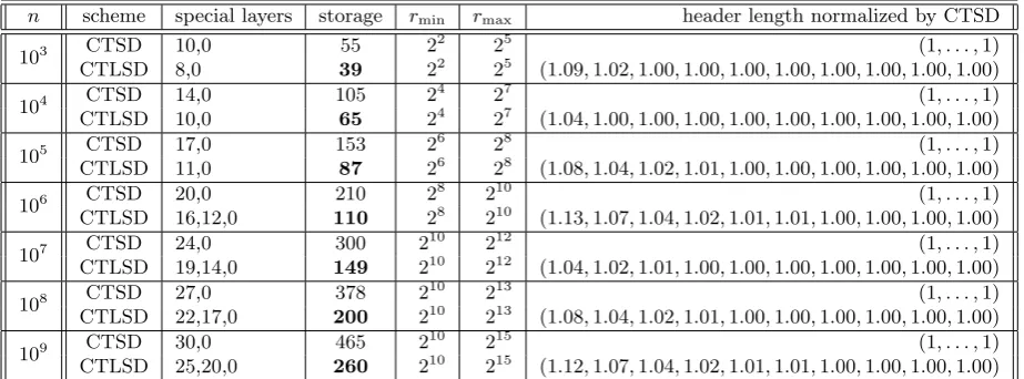
Table 6 provides some examples of running the algorithm for computing expected header length for non-full trees using the CTSD and the CTLSD schemes. The chosen values of r are 10 equispaced values between rmin
n scheme special layers storage rmin rmax header length normalized by CTSD
103 CTSD 10,0 55 2
2
25 (1, . . . ,1)
CTLSD 8,0 39 22 25 (1.09,1.02,1.00,1.00,1.00,1.00,1.00,1.00,1.00,1.00)
104 CTSD 14,0 105 2
4 27 (1, . . . ,1)
CTLSD 10,0 65 24 27 (1.04,1.00,1.00,1.00,1.00,1.00,1.00,1.00,1.00,1.00)
105 CTSD 17,0 153 2
6
28 (1, . . . ,1)
CTLSD 11,0 87 26 28 (1.08,1.04,1.02,1.01,1.00,1.00,1.00,1.00,1.00,1.00)
106 CTSD 20,0 210 2
8 210 (1, . . . ,1)
CTLSD 16,12,0 110 28 210 (1.13,1.07,1.04,1.02,1.01,1.01,1.00,1.00,1.00,1.00)
107 CTSD 24,0 300 2
10
212 (1, . . . ,1)
CTLSD 19,14,0 149 210 212 (1.04,1.02,1.01,1.00,1.00,1.00,1.00,1.00,1.00,1.00)
108 CTSD 27,0 378 2
10 213 (1, . . . ,1)
CTLSD 22,17,0 200 210 213 (1.08,1.04,1.02,1.01,1.00,1.00,1.00,1.00,1.00,1.00)
109 CTSD 30,0 465 2
10
215 (1, . . . ,1)
[image:20.595.68.530.91.262.2]CTLSD 25,20,0 260 210 215 (1.12,1.07,1.04,1.02,1.01,1.01,1.00,1.00,1.00,1.00)
Table 6: Comparison of the storage and the expected header lengths for the CTSD and the CTLSD (with constrained minimization layering) schemes.
Since the CTLSD scheme subsumes the HS LSD and the e-HS LSD schemes, this algorithm computes the expected header length for these schemes too. In [6], it was mentioned that the expected header length for their layering scheme, i.e; HS layering is around 2r. As we have seen earlier, by suitably placing the special levels, this can be brought down significantly to about the expected header length of the SD scheme. On the other hand, for the (e-)HS scheme, the expected header length can also be somewhat larger than 2r. For example, for l0 = 28 and r= 2, the expected header length is 2.23r.
5
Conclusion
In this work, we have suggested new layering strategies for the SD scheme. At one end we have shown that it is possible to decrease the user storage below that obtained by Halevy and Shamir [6]. At the other end, we have shown that it is possible to attain header length very close to that of the SD scheme while still requiring a significantly smaller number of keys. The LSD scheme is extended to handle arbitrary number of users leading to the CTLSD scheme. We have obtained an efficient algorithm to compute the expected header length in the CTLSD scheme. Our analysis of different scenarios is made possible by using this algorithm.
Acknowledgement
We would like to thank the anonymous reviewers for their comments and suggestions which has helped to improve the paper.
References
[1] Shimshon Berkovits, “How to broadcast a secret,” in EUROCRYPT, Donald W. Davies, Ed. 1991, vol. 547 ofLecture Notes in Computer Science, pp. 535–541, Springer.
[2] Amos Fiat and Moni Naor, “Broadcast encryption,” in CRYPTO, Douglas R. Stinson, Ed. 1993, vol. 773 ofLecture Notes in Computer Science, pp. 480–491, Springer.