SRC RR 133A pdf

December 30, 1994

SRC

Research

Report

133a

The Third Annual Video Review

of Computational Geometry

Edited by Marc H. Brown and John Hershberger

d i g i t a l

Systems Research Center 130 Lytton Avenue

Systems Research Center

The charter of SRC is to advance both the state of knowledge and the state of the art in computer systems. From our establishment in 1984, we have performed ba-sic and applied research to support Digital’s business objectives. Our current work includes exploring distributed personal computing on multiple platforms, network-ing, programming technology, system modelling and management techniques, and selected applications.

Our strategy is to test the technical and practical value of our ideas by building hard-ware and softhard-ware prototypes and using them as daily tools. Interesting systems are too complex to be evaluated solely in the abstract; extended use allows us to investi-gate their properties in depth. This experience is useful in the short term in refining our designs, and invaluable in the long term in advancing our knowledge. Most of the major advances in information systems have come through this strategy, includ-ing personal computinclud-ing, distributed systems, and the Internet.

We also perform complementary work of a more mathematical flavor. Some of it is in established fields of theoretical computer science, such as the analysis of algo-rithms, computational geometry, and logics of programming. Other work explores new ground motivated by problems that arise in our systems research.

We have a strong commitment to communicating our results; exposing and testing our ideas in the research and development communities leads to improved under-standing. Our research report series supplements publication in professional jour-nals and conferences. We seek users for our prototype systems among those with whom we have common interests, and we encourage collaboration with university researchers.

The Third Annual Video Review

of Computational Geometry

Edited by Marc H. Brown and John Hershberger

Author Affiliation

John Hershberger is currently employed by Mentor Graphics. He can be reached at

[email protected].

c

Digital Equipment Corporation 1994

The copyright of each section in this report is held by the author of the section. Sim-ilarly, the copyright of each segment of the accompanying videotape is held by the contributor of the segment. All other material in the report is copyrighted cDigital

Abstract

Computational geometry concepts are often easiest to understand visually, in terms of the geometric objects they manipulate. Indeed, most papers in the field rely on diagrams to communicate the intuition behind their results. However, static figures are not always adequate.

Preface

Computational geometry concepts are often easiest to understand visually. Indeed, most papers in computational geometry rely on diagrams to communicate the in-tuition behind their results. However, static figures are not always adequate to de-scribe geometric algorithms, since algorithms are inherently dynamic. The accom-panying videotape showcases advances in the use of algorithm animation, visual-ization, and interactive computing in the study of computational geometry.

This report contains short descriptions of the eight segments in the videotape. The first three segments are animations of two-dimensional algorithms: a polygonal approximation algorithm from cartography, an algorithm for computing the rectan-gle discrepancy, and a fixed-radius neighbor-searching algorithm. The fourth seg-ment presents the GASP system for animating geometric algorithms in two or three dimensions; GASP is used by two other segments in the review. The remaining segments illustrate algorithms and concepts in three or more dimensions: the fifth segment explores the relationship between penumbral shadows in three dimensions and four-dimensional polytopes; the final three segments show three-dimensional algorithms for interactive collision detection, polyhedral separators, and interactive display of alpha hulls.

This report and the accompanying videotape comprise the Third Annual Video Review of Computational Geometry. In the three years since the Video Review was introduced, it has become an established part of the annual ACM Symposium on Computational Geometry. The 1995 Video Review and future editions will be dis-tributed by the ACM as part of the conference proceedings.

We thank Bob Taylor, director of the Systems Research Center, for his support in establishing the annual Video Review. The ’92 Video Review is available as SRC Research Report 87, and the ’93 Video Review as SRC Research Report 101. These reports (written guides and videotapes) are available by sending electronic mail to

[email protected].

Finally, we thank the members of the 1994 Video Program Committee for their help in evaluating the entries. The members of the committee were Marshall Bern (Xerox PARC), Marc Brown (Digital Equipment Corporation’s Systems Research Center), Leo Guibas (Stanford University), John Hershberger (Mentor Graphics), Jim Ruppert (NASA Ames), and Jenny Zhao (Silicon Graphics).

Marc H. Brown John Hershberger

Table of Contents

Starting

Time

Title and Author

Page

1

2:17 An

O

(

n

log

n

)

Implementation of the Douglas-Peucker 1 Algorithm for Line Simplification

John Hershberger and Jack Snoeyink

2

7:15 Computing the Rectangle Discrepancy 5

David Dobkin and Dimitrios Gunopulos

3

14:38 An Animation of a Fixed-Radius All-Nearest Neighbors Algorithm 9 Hans-Peter Lenhof and Michiel Smid

4

22:29 GASP–A System to Facilitate Animating Geometric Algorithms 11 Ayellet Tal and David P. Dobkin

5

30:42 Penumbral Shadows 18

Adrian Mariano and Linus Upson

6

33:54 Exact Collision Detection for Interactive Environments 20 J. D. Cohen, M. C. Lin, D. Manocha, and M. K. Ponamgi

7

40:36 Almost Optimal Polyhedral Separators 25

Herv´e Br¨onnimann

An

O(nlogn)

Implementation

Of The Douglas-Peucker Algorithm

For Line Simplification

John Hershberger

Mentor Graphics

1001 Ridder Park Drive

San Jose, CA 95131

Jack Snoeyink

Department of Computer Science

University of British Columbia

Vancouver, BC V6T 1Z2 Canada

1

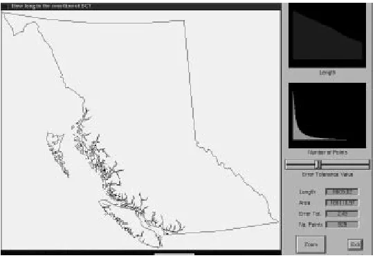
The “line simplification problem” is as follows: Given a sequence of vertices that make up a polygonal chain, find a subsequence of the vertices that approximates the chain. The accompanying videotape shows two algorithms for solving the line simplification problem.

Introduction

An important task of the cartographer’s art is to extract features from detailed data and represent them on a simple and readable map. As computers become increas-ingly involved in automated cartography, efficient algorithms are needed for the tasks of extraction and simplification. Cartographers [1, 6] have identified the line simplification problem as an important part of representing linear features. Given a polygonal chain, a sequence of vertices

V

=

f

v

0

;v

1

;:::;v

n

g, the problem is to

find a subsequence of vertices that approximates the chain

V

. We assume that the input chain

V

has no self-intersections (but not the output).

[image:9.612.190.461.134.321.2]

1

Figure 1: Simplifying the polygonal chain representing the coastline of British Columbia.

as vision [8] and computational geometry [9]. The accompanying videotape ani-mates two different implementations of this simplification method—the straightfor-ward implementation suggested by Douglas and Peucker and the implementation of Hershberger and Snoeyink that improves the worst-case running time.

Method

Given a polygonal chain

V

=

f

v

0

;v

1

;:::;v

n

g, the recursive line simplification

method proceeds as follows: Initially, approximate

V

by the line segment

v

0

v

n

.

Determine the farthest vertex

v

f

from the line

v

!

0

v

n

. If its distance

d

(

v

f

;

!

v

0

v

n

)

is

at most a given tolerance

"

0

, then accept the segment

v

0

v

n

as a good

approxi-mation to

V

. Otherwise, break

V

at

v

f

and recursively approximate the subchain

f

v

0

;v

1

;:::;v

f

gandf

v

f

;:::;v

n

g.

Algorithms

The two implementations differ in the way they find

v

f

, the farthest vertex from

!

1

The straightforward approach measures distance from

v

!

0

v

n

for each vertex and

takes the maximum. Thus, the running time of this algorithm will satisfy a quicksort-like recurrence, with best case

(

n

log

n

)

. Since geometry determines the farthest vertex, the worst-case running time is

(

n

2

)

. One cannot use linear-time median finding or randomization to improve the running time. (If one assumes that the in-put data is such that farthest vertices are found near the middle of chains, then one expects

O

(

n

log

n

)

behavior.)

The second implementation uses a path hull data structure [2, 4] to maintain a dynamic convex hull of the polygonal chain

V

. Using Melkman’s convex hull al-gorithm [7], we compute two convex hulls from the middle of the chain outward. We can find a farthest vertex

v

f

from a line by locating two extreme points on each hull using binary search. When we split

V

at vertex

v

f

, we undo one of the hull computations to obtain the hull from the “middle” to

v

f

, recursively approximate the subchain containing the middle, then build hulls for the other subchain and re-cursively approximate it. One can use a simple credit argument to show that the total time taken by the algorithm is

O

(

n

log

n

)

. The best case can even be linear, if all the hulls are small and splits occur at the ends.

Unfortunately for us, the statistical properties of cartographic data usually mean that the straightforward implementation is slightly faster than the path hull imple-mentation. Since the variance of the running time of the path hull implementation is smaller, it may be interesting for parallel or interactive applications.

Technical Details

The programs were run on a Silicon Graphics Crimson in the GraFiC lab at UBC and output was recorded to video in real time.

Acknowledgments

1

References

[1] B. Buttenfield. Treatment of the cartographic line. Cartographica, 22:1–26, 1985.

[2] D. Dobkin, L. Guibas, J. Hershberger, and J. Snoeyink. An efficient algorithm for finding the CSG representation of a simple polygon. Algorithmica, 10:1– 23, 1993.

[3] D. H. Douglas and T. K. Peucker. Algorithms for the reduction of the number of points required to represent a line or its caricature. The Canadian Cartog-rapher, 10(2):112–122, 1973.

[4] J. Hershberger and J. Snoeyink. Speeding up the Douglas-Peucker line sim-plification algorithm. In Proc. 5th Intl. Symp. Spatial Data Handling, pages 134–143. IGU Commission on GIS, 1992.

[5] R. B. McMaster. A statistical analysis of mathematical measures for linear simplification. Amer. Cartog., 13:103–116, 1986.

[6] R. B. McMaster. Automated line generalization. Cartographica, 24(2):74– 111, 1987.

[7] A. A. Melkman. On-line construction of the convex hull of a simple polyline. Info. Proc. Let., 25:11–12, 1987.

[8] U. Ramer. An iterative procedure for the polygonal approximation of plane curves. Comp. Vis. Graph. Image Proc., 1:244–256, 1972.

[9] G. Rote. Quadratic convergence of the sandwich algorithm for approximating convex functions and convex figures in the plane. In Proc. 2nd Can. Conf. Comp. Geom., pages 120–124, Ottawa, Ontario, 1990.

Computing the Rectangle Discrepancy

David P. Dobkin and Dimitrios Gunopulos

Department of Computer Science

Princeton University

Princeton, NJ 08544

2

Supersampling is one of the most general ways of attacking the problem of antialias-ing in computer graphics. In this approach, a picture is sampled at a very high rate, and then resampled by averaging supersamples within the pixel area to compute the pixel value. Ray tracing, a common technique used to produce realistic images of computer modeled scenes, is another instance of supersampling. Discrepancy the-ory provides a measure of the quality of the sampling patterns. The “rectangle dis-crepancy” in particular gives a good measure of how well a sample pattern, when applied to the area of one or more pixels, captures small details in the picture. The accompanying videotape shows an animation of an algorithm we have developed [2] for computing the “rectangle discrepancy” of a two-dimensional point set. In particular, this algorithm can be used to find sampling sets with very low rectangle discrepancy. Interestingly the problem of computing the rectangle discrepancy also arises in the context of learning theory [4].

Definitions

Let us consider a point setX in the unit square. LetF be the set of all rectangles in

the unit square with edges parallel to the two axes. For an axis-oriented rectangle

A

(

A

2F), we define the function

[image:13.612.188.461.134.340.2]

2

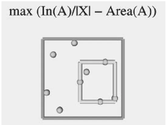
Figure 2: The rectangle that maximizesD

l

.

The rectangle discrepancy of a rectangle

A

2Fis

D

(

A

) =

j

In

(

A

)

=

jXj

Area

(

A

)

j

The maximum rectangle discrepancy of the setX is

Max

D

(

X

) =

max

A

2F

(

D

(

A

))

We also define the following simpler functions for

A

2F

D

l

(

A

) =

In

(

A

)

=

jXj

Area

(

A

)

and

D

o

(

A

) =

Area

(

A

)

In

(

A

)

=

jXj

The algorithm we present in this animation computes

Max

D

l

(

X

) =

max

A

2F

(

D

l

(

A

))

for a given input setX, in time

O

(

jXj 2

log

jXj

)

. The same techniques however can

2

Videotape Contents

We explain the main idea of the algorithm in a series of simple lemmata. First we show that we have to consider at most

O

(

jXj

4

)

rectangles, more specifically the ones that have all their edges pass through a point inX.

This allows us to study pairs of points in in X. For each such pair we find

the rectangle that maximizesD

l

over all rectangles with horizontal edges that pass

through the points of the given pair.

This problem is much easier now because we know the

y

coordinates of the rectangle. Assuming that the two points are

p

b

;p

t

(

p

b

(

y

)

< p

t

(

y

)

), and the height of the rectangle is

dy

, (

dy

=

p

t

(

y

)

p

b

(

y

))

we have to find the following maximum

max

A

2F

ij

(

In

(

A

)

=

jXj

dx

A

dy

)

whereF

ij

is the set of rectangles that pass through points

p

b

and

p

t

, and

dx

A

is the

width of

A

. If we eliminate the points inXthat either lie above the top

y

coordinate

of the rectangle or below the lower

y

coordinate, this becomes a one-dimensional problem. We project the points on the

x

axis and obtain a new setX

0

of one-dimensional points. We can equivalently maximize the following function

max

A

2[0

;

1]

;p

b

(

x

)2

A

(

In

(

A

)

=

jX

0

j

Length

(

A

))

We can reduce this problem to the problem of computing the halfspace discrepancy of one-dimensional point sets, a simpler problem studied in [1]. Here we want to find the anchored interval that maximizes

max

A

=[0

;z

i

]

(

i=

jZj

z

i

)

for a given one-dimensional setZ

=

f

z

1

:::z

n

gwith

0

z

i

< z

i

+1

1

. This

is a linear function of the rank and the coordinate of the point. To solve it we find the convex hull of the setf

(

z

1

;

1)

:::

(

z

n

;n

)

gand find the maximum with a binary

search. From this maximum we obtain the solution to the original maximization problem.

In this way we compute the maximum rectangle for all pairs of points. Clearly the rectangle that maximizesD

l

is the maximum of these

O

(

jXj

2

)

rectangles. Finally, we show how to use the dynamic data structure of [5] to solve a se-quence of one-dimensional problems efficiently. With the use of this technique we can maintain the convex hull at a cost of

O

(log

2

jXj

)

time per insertion. This in

turn allows us to find the maximum rectangle for each pair of points in

O

(log

2 jXj

)

time, and yields the final running time of

O

(

jXj 2

log

2

Technical Details

The accompanying videotape was prepared in the Computer Science Department at Princeton University. The implementation of the algorithm was written in C, to run under UNIX on a Silicon Graphics Iris workstation. The animation was created with the animation system GASP that Ayellet Tal and David Dobkin are developing in this department [3]. Recording was done at the Interactive Computer Graphics Lab at Princeton and editing was done with the assistance of the Department of Me-dia Services at Princeton.

Acknowledgments

This work supported in part by the National Science Foundation under Grant Num-ber CCR93-01254 and by The Geometry Center, University of Minnesota, an STC funded by NSF, DOE, and Minnesota Technology, Inc.

References

[1] D.P. Dobkin and D. Eppstein, Computing the Discrepancy. Proceedings of the Ninth Annual Symposium on Computational Geometry, (1993).

[2] D.P. Dobkin and D. Gunopulos, Computing the Rectangle Discrepancy. Prince-ton University Technical Report 443-94.

[3] D.P. Dobkin and A. Tal, GASP – A System to Facilitate Animating Geomet-ric Algorithms. Third Annual Video Review of Computational Geometry, to ap-pear, (1994)

[4] W. Maass, Efficient Agnostic PAC-Learning with Simple Hypotheses. Submit-ted to COLT ’94.

An Animation of a Fixed-Radius All-Nearest

Neighbors Algorithm

Hans-Peter Lenhof and Michiel Smid

Max-Planck-Institut f¨ur Informatik

D-66123 Saarbr¨ucken, Germany

3

A fixed-radius all-nearest neighbors problem takes as input a set

S

of

n

points and a real number

, and reports all pairs of points that are at distance at most

. The accompanying videotape shows an animation of an algorithm, developed by the au-thors [2], for solving the fixed-radius all-nearest neighbors problem.

The Algorithm

The algorithm depicted in the videotape works in two stages. In the first stage, a grid is computed. Instead of a standard grid, we use a so-called degraded grid that is easier to construct by means of a simple sweep algorithm. This degraded grid consists of boxes with sides of length at least

. If a box contains points of

S

, then its sides are of length exactly

. In the second stage, this grid is used for the actual enumeration. For each non-empty box, it suffices to compare each of its points with all points in the same box or in one of the neighboring boxes. Although the algo-rithm may compare many pairs having distance more than

, it can be shown that the total number of pairs considered is proportional to the number of pairs that are at most

apart. As a result, the total running time of the algorithm is proportional to

n

log

n

plus the number of pairs that are at distance at most

.

3

for a suitable choice of

. This gives for each point a neighbor list containing all points that are at distance at most

from it. Given these lists, we can triangulate the surface incrementally: An edge of the current triangulation is called an outer edge, if it belongs to only one triangle. All outer edges are maintained in a queue. With each edge, we store a so-called common neighbor list, which is the intersection of the two neighbor lists of the points belonging to this edge. We start with any triangle. Its edges and their common neighbor lists are inserted into the queue. As long as the queue is non-empty, we do the following: We take any edge from the queue and look at all points in its common neighbor list. Each such point defines a triangle with the current edge. We take that point defining the smallest triangle. This triangle becomes part of the triangulation and we update the queue appropriately.

Technical Details

The video was produced at the Max-Planck-Institute for Computer Science, using Silicon Graphics Indy and Indigo2

machines, and using Showcase and Geomview-1.1 software. We thank Roland Berberich, Jack Hazboun, Dirk Louis and Peter M¨uller for their help in producing this video.

Acknowledgments

This work was supported by the ESPRIT Basic Research Actions Program, under contract No. 7141 (project ALCOM II).

References

[1] W. Heiden, M. Schlenkrich and J. Brickmann. Triangulation algorithms for the representation of molecular surface properties. J. Comp. Aided Mol. Des. 4 (1990), pp. 255-269.

GASP - A System to Facilitate Animating

Geometric Algorithms

Ayellet Tal and David Dobkin

Department of Computer Science

Princeton University

Princeton, NJ 08544

4

The accompanying videotape shows five algorithm animations that have been de-veloped using GASP. The GASP system is noteworthy because it is very easy for a user without any knowledge of computer graphics to create an animation of a geo-metric algorithm quickly.

Overview

The GASP system helps in the creation and viewing of animations for geometric algorithms. The user need not have any knowledge of computer graphics in order to quickly generate an animation. GASP allows the fast prototyping of algorithm animations. A typical animation can be produced in a matter of days or even hours. Even highly complex geometric algorithms can be animated with ease. The system is also intended to facilitate the task of implementing and debugging geometric al-gorithms.

[image:19.612.188.461.133.349.2]

4

Figure 3: Polyhedral Hierarchies

knowledge of computer graphics. The animation is generated automatically by the system. But a different animation will be generated if the style file is modified.

The GASP environment allows the viewer to control the execution of the al-gorithm in an easy way. The animation can be run at varying speeds: fast(

>>

), slow(

>

) or step by step (

>

j). The analogous

<

,

<<

and j

<

push buttons run

the algorithm in reverse. The viewer can PAUSE at any time to suspend the execu-tion of the algorithm or can EJECT the movie. The environment is invaluable for education and debugging.

Videotape Contents

4

Clip 1: Polyhedral Hierarchies

To begin, we show a clip from [6]. This is the hierarchical data structure for rep-resenting convex polyhedra [4, 5], and the animation was an aid in debugging the algorithm for detecting plane-polyhedral intersection. We explain a single pluck and then show how the hierarchy progresses from level to level. To create the an-imation for explaining a single pluck the user need only write the following short code:

explain_pluck(poly_vert_no, poly_vertices, poly_face_no, poly_faces, poly_names, vert_no, vertices, face_no, faces) {

/* create the polyhedron */ Begin_atomic("poly"); Create_polyhedron("P0",

poly_vert_no, poly_face_no, poly_vertices, poly_faces); Rotate_world();

End_atomic();

/* remove vertices and cones */ Begin_atomic("pluck");

Split_polyhedron(poly_names, "P0", vert_no, vertices); End_atomic();

/* add new faces */

Begin_atomic("add_faces");

Add_faces(poly_names[0], face_no, faces); End_atomic();

/* undo plucking */ Undo(2);

4

Clip 2: Objects That Cannot Be Taken Apart With Two Hands

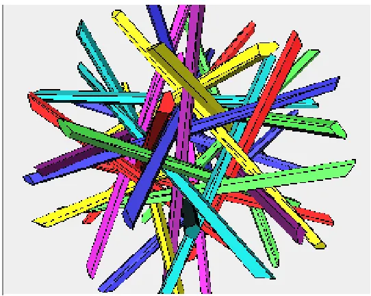
The second animation, based on [10], is a remake of [9]. The animation shows a configuration of six tetrahedra that cannot be taken apart by translation with two hands. Then, it presents a configuration of thirty objects that cannot be taken apart by applying an isometry to any proper subset. The purpose of the animation is to illustrate the use of GASP as an illustration tool for geometric configurations. It took us far less than a day to generate that animation. The animation was created by the following function:

hands(){

for (i = 0; i < stick_no; i++){ /* stick i */

get_polyhedron(&points,

&indices, &nmax, &fmax, &atomic_name, &stick_name); Begin_atomic(atomic_name);

Create_polyhedron(stick_name, nmax, fmax, points, indices); End_atomic();

}

Begin_atomic("Rotate"); Rotate_world();

End_atomic(); }

4

begin_global_style

background = 0.9 0.9 0.9; color = VIDEO;

frames = 10; end_global_style

begin_unit_style Rotate frames = 160;

rotation_world = Y 380.0; end_unit_style

begin_unit_style stick0

[image:22.612.151.422.398.614.2]

color = 0.625 0.273475 0.273475; end_unit_style

4

Clip 3: Motion Planning

Next we show an animation of a motion planning algorithm [7]. It is a repeat of the first part of [8]. The object to be moved is a disc and the obstacles are simple disjoint polygons. The goal of the animation is to show the use of GASP in creating two-dimensional animations.

Clip 4: Line Segment Intersection

The fourth animation, which is based on [2], shows a line segment intersection al-gorithm in action and illustrates its most important features. The animation consists of three phases. The first phase presents the initial line segments and the visibility map that needs to be built. The second phase demonstrates that the visibility map is being constructed by operating in a sweepline fashion, scanning the segments from left to right, and maintaining the vertical visibility map of the region swept along the way. The third phase demonstrates that the cross section along the sweepline is maintained in a lazy fashion. The animation is used as an aid in explaining a highly complex algorithm and to allow students to interact with the algorithm. A student can choose the initial line segments by editing an ASCII file and view how the an-imation is changing.

Clip 5: Heapsort

The last clip animates heapsort. The colored rods have lengths to be sorted. We first display the initial creation of the heap. Next, simple motions are used to control the repeated operations of removing the largest element, and reheaping. Heapsort is given as an example of using GASP to facilitate the animation of any algorithm that involves the display of three dimensional geometries.

Technical Details

4

Acknowledgments

We thank Kirk Alexander and Mike Mills for their help in producing the final video. This work supported in part by the National Science Foundation under Grant Num-ber CCR93-01254 and by The Geometry Center, University of Minnesota, an STC funded by NSF, DOE, and Minnesota Technology, Inc.

References

[1] H. Bronnimann. Almost optimal polyhedral separators. In The Third Annual Video Review of Computational Geometry, 1994.

[2] B. Chazelle and H. Edelsbrunner. An optimal algorithm for intersecting line segments in the plane. Journal of the ACM, 39(1):1–54, 1992.

[3] D. Dobkin and D. Gunopulos. Computing the rectangle discrepancy. In The Third Annual Video Review of Computational Geometry, 1994.

[4] D. Dobkin and D. Kirkpatrick. Fast detection of polyhedral intersections. Journal of Algorithms, 6:381–392, 1985.

[5] D. Dobkin and D. Kirkpatrick. Determining the separation of preprocessed polyhedra – a unified approach. ICALP, pages 400–413, 1990.

[6] D. Dobkin and A. Tal. Building and using polyhedral hierarchies (video). In The Ninth Annual ACM Symposium on Computational Geometry, page 394, May 1993.

[7] H. Rohnert. Moving a disc between polygons. Algorithmica, 6:182–191, 1991.

[8] S. Schirra. Moving a disc between polygons (video). In The Ninth Annual ACM Symposium on Computational Geometry, pages 395–396, May 1993.

[9] J. Snoeyink. Objects that cannot be taken apart with two hands (video). In The Ninth Annual ACM Symposium on Computational Geometry, page 405, May 1993.

Penumbral Shadows

Adrian Mariano

Center for Applied Math

Cornell University

Ithaca, NY 14853–3801

Linus Upson

NeXT

900 Chesapeake Drive

Redwood City, CA 94063

5

The shadows cast by polygonal occluding objects illuminated by polygonal light sources are complicated. Unlike shadows cast by point sources, they are divided into regions where the shadow intensity changes at different rates. The boundaries between these different regions form the shadow diagram.

The accompanying videotape depicts shadows cast by a square light source with a square occluding object. We have included two types of images: flat shadow scenes and perspective views. The flat shadow images were calculated using the exact formula for radiative energy transfer. This calculation depends only on the boundary of the visible light source. For polygons, it can be reduced to a simple summation [1].

Finding the boundary of the visible portion of the illuminating polygon when it is occluded by a second polygon requires computing the intersection of two poly-gons. General purpose algorithms for computing intersections of arbitrary polygons in the plane are quite complicated, so we used the Sutherland–Hodgman algorithm, which cannot handle concave polygons, but which is much simpler than the fully general methods [2]. We created the three-dimensional perspective views from the flat images using the texture mapping capabilities of Rayshade.

5

In general, the shadow diagrams for an arbitrary light source and occluder can be seen as projections of four-dimensional polytopes by considering the lines which intersect the plane of the shadow. Let

S

be the plane of the shadow and let

P

be a different plane parallel to

S

. If a line intersects

S

at the point

(

x

s

;y

s

)

and it inter-sects

P

at the point

(

x

p

;y

p

)

then the line can be mapped to a point

(

x

s

;y

s

;x

p

;y

p

)

in R4

. Now let

D

be the set of all lines which intersect both the light source and the occluder. When

D

is mapped into R4

, the result is a four-dimensional polytope. If this polytope is projected into R2

by discarding the last two coordinates of each point, the shadow diagram results. Because

P

can be changed, this construction describes a particular shadow diagram as the projections of any one of a family of polytopes.

References

[1] Hottel and Sarofim. Radiative Transfer. McGraw Hill, New York. 1967.

[2] Vatti, Bala. “A Generic Solution to Polygon Clipping.” Communications of the ACM, July 1992.

Exact Collision Detection for

Interactive Environments

Jonathan D. Cohen

Dinesh Manocha

Madhav K. Ponamgi

Computer Science Department

University of North Carolina

Chapel Hill, NC 27599-3175

Ming C. Lin

Computer Science Department

Naval Postgraduate School

Monterey, CA 93943

6

The accompanying videotape demonstrates algorithms for collision detection in large-scaled, interactive environments. Such environments are characterized by the num-ber of objects undergoing rigid motion and the complexity of the models. The algo-rithms do not assume that the motions of the objects are expressible as closed form functions of time, nor do they assume any upper bounds on their velocities.

Background

Over the last few years, a great deal of interest has been generated in virtual or synthetic environments, such as architectural walkthroughs, visual simulation sys-tems for designing the shapes of mechanical parts, training syssys-tems, etc. Interac-tive, large-scaled virtual environments pose new challenges to the collision detec-tion problem, because they require performance at interactive rates for thousands of pairwise intersection tests [1].

[image:28.612.206.369.135.297.2]

reduc-6

Figure 5: An example of collision detection for convex poly-hedra

tion approach (based on a technique termed as sweep and prune) and the temporal and geometric coherence that exists between successive frames to overcome the bottleneck of

O

(

n

2

)

pairwise comparison tests in a large environment of

n

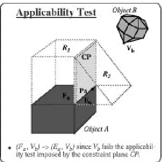
moving objects [1]. After we eliminate the object pairs that are not in the close vicinity of each other, we employ an exact collision detection scheme. The exact convex poly-tope collision detection algorithm is based upon [2]: locality (captured by walking from one Voronoi region of the candidate feature to one of its neighboring features’ Voronoi regions according to the constraints failed) and coherence (used to reduce computation efforts in a dynamic environment). We can deal with non-convex ob-jects or articulated bodies by using a sub-part hierarchical tree representation.

Exact Collision Detection

The Voronoi regions form a partition of space outside the polytope according to the closest feature. The collection of Voronoi regions of each polytope is the general-ized Voronoi diagram of the polytope. Note that the generalgeneral-ized Voronoi diagram of a convex polytope has linear size and consists of polyhedral regions. Each Voronoi region is bounded by a set of constraint planes with pointers to the neighboring cells (which each share a constraint plane with it).

6

which share this constraint plane in their Voronoi regions. If a point

P

on object

A

lies inside the Voronoi region of the feature

f

B

on object

B

, then

f

B

is a closest feature to the point

P

.

Our method is straightforward. We start with a candidate pair of features, one from each polytope, and check whether the closest points lie on these features. Since the polytopes and their faces are convex, this is a local test involving only the neigh-boring features of the current candidate features. If either feature fails the test, we step to a neighboring feature of one or both candidates, and try again. With some simple preprocessing, we can guarantee that every feature has a constant number of neighboring features. This is how we can verify or update the closest feature pair in expected constant time. Fig. 5 shows how this algorithm works on a pair of simple convex polytopes.

Sweep and Prune

The exact polytope collision detection algorithm is fast enough to perform collision detection at real-time, in a multi-body environment of moderate size. However, the

O

(

n

2

)

pairwise detection tests become a bottleneck for large

n

. By exploiting the spatial and temporal coherence, we use a method whose running time is a linear function of the number of objects and the number of pairs of objects in close vicinity of each other.

For each object in the environment, we compute a smallest fitting, axis-aligned bounding box, which is dynamically resized using a hill-climbing algorithm based on the properties of convex polytopes and the principle of coherence.

These bounding boxes are used to prune down the number of pairwise collision detection tests. We take the orthogonal projections of the bounding boxes onto the

x

,

y

, and

z

axes and sort the intervals in three separate lists. If the projections over-lap in all three dimensions, we activate the exact collision detection algorithm. At each frame, we sweep over the sorted lists of intervals, updating them and culling out the pairs of non-overlapping bounding boxes.

6

Video Contents

We have successfully demonstrated the algorithm in an architectural walkthrough environment and a multi-body simulation system. For simulations consisting of thousands of models, the overall algorithm has exhibited linear time performance in practice.

We first demonstrate how the polytope collision detection algorithm [2] tracks the closest features between two convex polytopes in real time. We maintain and update the closest features using the Voronoi regions of the polytopes. Since the polytopes move only slightly between the frames, the temporal and geometric co-herence is well preserved. Thus, the expected running time of this algorithm is con-stant, independent of the complexity of the polytopes.

This is followed by demonstrating the algorithm on an articulated body, namely a hand, represented by the union of multiple convex polytopes. To demonstrate the efficiency of the algorithm and effectiveness of the coherence, we keep track of all pairs of closest features between each finger and the nearby objects. However, using a subpart hierarchical tree representation as in [2] can eliminate the unnecessary computation.

The over all collision detection algorithm is tested on a walkthrough and a multi-body dynamic simulation environment. The video footage of walkthrough was taken from a user’s actual walkthrough experience. The collision detection algorithm performs very well in large environments composed of hundreds of polytopes. The kitchen, like most realistic environments, is fairly static; therefore, we can sort the bounding boxes of the polytopes in sub-linear time at each instance (this requires a modified sorting algorithm which sorts only the moving objects). We see very little degradation of frame rate when we add the capability of collision detection to our walkthrough environment.

6

Acknowledgments

We are grateful to Dr. Fred Brooks and the walkthrough group at UNC Chapel Hill for the model of the kitchen.

D. Manocha was supported in part by a Junior Faculty Award and ARPA Con-tract #DAEA 18-90-C-0044.

References

[1] J. Cohen, M. Lin, D. Manocha, and K. Ponamgi. Interactive and exact collision detection for large-scaled environments. Technical Report TR94-005, Depart-ment of Computer Science, University of North Carolina, 1994.

Almost Optimal Polyhedral Separators

Herv´e Br¨onnimann

Department of Computer Science

Princeton University

Princeton, NJ 08544

7

The accompanying videotape illustrates two deterministic polynomial time methods for finding a separator for two nested convex polyhedra in 3-dimensions.

1

Introduction

Let

Q

P

be two convex polyhedra in IR 3

. The problem of finding a separating convex polyhedron between

P

and

Q

with as few facets as possible is believed to be NP-hard [2], but one can find good approximations for it. Mitchell and Suri [4] cast the problem as a set cover problem. LetH

=

H

(

Q

)

denote the set of supporting

hyperplanes of

Q

. Let the cover set system be

(

H

;

fH

p

:

p

2

@P

g

)

, where, for any

point

p

,H

p

consists of those hyperplanes inHfor which

p

and

Q

lie on opposite

sides. They show that a hitting set for the cover set system gives a subset of facets of

Q

whose supporting halfspaces define a polytope whose boundary lies between

Q

and

P

.

A polytope

Q

0

between

Q

and

P

such that each facet of

Q

0

7

2

Video Contents

We first familiarize the viewer with the two polyhedra

Q

P

;

Q

is seen inside

by means of transparency (see Fig. 6, top). We explain how to obtain canonical separators, and how to construct the set system. The portion of the arrangementA

ofH

(

Q

)

on the boundary of

P

is visualized, and some rows of the set system are

then shown sequentially, one corresponding to each facet of this arrangement. To explain the greedy method on this set system, an approach which is proposed by Mitchell and Suri [4], we show how the choice of a facet removes a portion of the boundary of

P

, and how the greedy method proceeds sequentially by choosing the facet which covers the biggest remaining portion (measured by the number of cells ofAit separates from

Q

). After four iterations, we skip to the final greedy separator,

which has 14 facets. In general, the greedy separator is guaranteed to have at most

s

opt

log

j

Q

jfacets, where

s

opt

is the size of an optimal canonical separator.

Another algorithm is then animated. It is the weighting method described by Goodrich and the author in [1]. We show how putting a weight on the faces of

Q

induces a weight for the cells of the arrangementA, and how keeping only the heavy

cells yields a separator which is nothing else than a

(1

=

2

c

)

-net for the planesH

(

Q

)

[image:34.612.151.422.108.610.2]

7

Figure 6: The top image shows two nested polyhedra. The bottom image shows the weighted algorithm in action. Specif-ically, the heavy cells are displayed in yellow on

P

, and the

7

3

Technical Details

Both algorithms are implemented and animated using GASP, a Geometric Anima-tion System created at Princeton University by Ayellet Tal and David Dobkin [3]. The implementation is written in C and runs on a Silicon Graphics Iris workstation. The algorithm is fully animated, in the sense that it produces an animation for any given data

P

and

Q

. The data used for the video were created with a random gener-ator of planes tangent to the sphere, then intersected to obtain

Q

, which was blown up to yield

P

.

Acknowledgments

We would like to thank Ayellet Tal and David Dobkin for the customized GASP en-vironment and their invaluable help. Thanks also go to Kirk Alexander and Kevin Perry, of Interactive Computer Graphics Lab at Princeton University and Mike Mills, of the Princeton Department of Media Services.

The author was supported in part by NSF Grant CCR-93-01254, the Geome-try Center, University of Minnesota, an STC funded by NSF, DOE, and Minnesota Technology Inc., and Ecole Normale Sup´erieure of Paris.

References

[1] H. Br¨onnimann and M. T. Goodrich. Almost optimal set covers in finite VC-dimension. In Proc. 10th ACM Sympos. Computational Geometry, pages 293– 302, 1994.

[2] G. Das. Approximation schemes in computational geometry. Ph.D. thesis, Uni-versity of Wisconsin, 1990.

[3] D. P. Dobkin and A. Tal. GASP–a system to facilitate animating geometric algorithms (Video). These proceedings.

Interactive Visualization of Weighted

Three-dimensional Alpha Hulls

Amitabh Varshney

Frederick P. Brooks, Jr.

William V. Wright

Department of Computer Science

University of North Carolina at Chapel Hill

Chapel Hill, NC 27599-3175

8

The accompanying videotape shows an interactive visualization of weighted three-dimensional

-hulls for static and dynamic spheres. The

-hull is analytically com-puted and represented by a triangulated mesh. The entire surface is comcom-puted and displayed in real-time at interactive rates. The weighted three-dimensional

-hulls are equivalent to smooth molecular surfaces of biochemistry. Biochemistry appli-cations of interactive computation and display of

-hulls or smooth molecular sur-faces are outlined.

Introduction

The

-hull has been defined as a generalization of the convex hull of point-sets by Edelsbrunner, Kirkpatrick, and Seidel [3, 4]. Given a set of points

P

, a ball

b

of radius

is defined as an empty

-ball if

b

\

P

=

. For

0

1, the

-hull of

P

is defined as the complement of the union of all empty

-balls [3]. It has been shown that it is possible to compute the

-hull of a set of points

P

from the Voronoi diagram of

P

. For

=

1the

-hull over the set of points

P

is the same

as their convex hull. Edelsbrunner and M ¨ucke [5] have defined the

-shape over

8

of the

-hull by straight edges and spherical caps by triangles. An

-shape of a set of points

P

is a subset of the Delaunay triangulation of

P

. Edelsbrunner [3] has extended the concept of

-shapes to deal with weighted points (i.e. spheres with possibly unequal radii) in three dimensions. An

-shape of a set of weighted points

P

w

is a subset of the regular triangulation of

P

w

.

The smooth molecular surface of a molecule is defined as the surface which an exterior probe-sphere touches as it is rolled over the spherical atoms of that molecule. This definition of a molecular surface was first proposed by Richards [7]. This sur-face is useful in studying the structure and interactions of proteins, in particular for attacking the protein-substrate docking problem. The analytic computation of the molecular surface was first done by Connolly [2].

Looking at the above definitions, one can see that the weighted

-hulls for three dimensions and the smooth molecular surface of a molecule with a probe-radius

have the same definitions. In this video we present the visualization of weighted

-hulls as used to define molecular surfaces.

Our Approach

Computation of

-hulls and

-shapes has traditionally been done by first construct-ing power diagrams or regular triangulations. Since these methods involve comput-ing the entire diagram or triangulation first and then cullcomput-ing away the parts that are not required, their complexity is

O

(

n

2

)

in time, where

n

is the number of points. This is worst-case optimal, since an

-shape in three dimensions could have a com-plexity of

(

n

2

)

.

However, when

-hulls are used as molecular surfaces, one can do better. Let

M

=

f

S

1

;:::;S

n

g, be a set of spheres, where each sphere,

S

i

, is expressed as a

pair

(

c

i

;r

i

)

,

c

i

being the center of the sphere and

r

i

being the radius of the sphere. Collections of spheres representing molecules have two interesting properties: (i) the minimum distance

d

ij

between any two centers

c

i

and

c

j

is greater than or equal to a positive constant

l

min

— the smallest bond-length in the molecule and (ii) the values of all the radii can be bounded from above and below by strictly positive values,

0

< r

min

r

i

r

max

. We take advantage of the first property to arrive

[image:38.612.161.413.141.360.2]

8

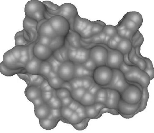
Figure 7: The molecular surface (alpha-hull) for crambin at probe-sphere radii (alpha value) of 1.4 ˚Angstroms.

A power cell (as described by Aurenhammer [1]) for a given sphere

S

i

with respect to

M

can be computed as the intersection of

n

1

halfspaces, each half-space contributed by the pair

(

S

i

;S

j

)

;

1

j

n;j

6

=

i

. If the average number

of neighbors for an atom is

k

, then for our purposes it is sufficient to just compute an approximation to the power cell, which we call a feasible cell, as an intersection of

k

halfspaces (one halfspace contributed by each neighbor). This can be done in deterministic time O(

k

log

k

). For

n

atoms, this task can be parallelized over

n

processors, each processor computing the feasible cell for one atom. To check if a feasible cell is non-null, we use a randomized linear programming algorithm that has linear expected time complexity and is quite fast in practice [8]. For details of our approach the interested reader can refer to [9].

8

of

1

:

4

A,˚

k

is around

45

.

In the algorithms for computing the convex hull of a set of points, it is assumed that the points are in a general position, i.e. no more than

d

points lie on the same

d

1

dimensional hyperplane. In reality this assumption often fails to hold, leading to problems. For example, planar benzene rings occur often in proteins, causing six carbon and six hydrogen atoms to be all coplanar. One of the recent approaches to solving this problem has been to perturb the input point set slightly to avoid these degeneracies. The approach of Emiris and Canny [6] perturbs the

j

th

dimension of the

i

th

point as:

p

i;j

(

) =

p

i;j

+

(

i

j

mod

q

)1

i

n;

1

j

d

(1)

where

is a symbolic infinitesimal and

q

is the smallest prime greater than

n

. In-stead of performing exact integer arithmetic, we just perturb the centers of the spheres by the above scheme and that has worked quite well for us in practice.

With no preprocessing, we can compute the molecular surface for a

396

atom Crambin and a probe-radius of

1

:

4

A, using˚

40

Intel i860 processors in 0.2 seconds. We have implemented

-hulls on Pixel-Planes 5, though the method is general enough to be easily implemented on any other parallel architecture. Our approach is analyt-ically exact. The only approximation is the degree of tessellation of spherical and toroidal patches.

Applications in Biochemistry

Interactive computation and display of molecular surfaces should benefit biochemists in three important ways. First, the ability to change the probe-radius interactively helps one study the surface. Second, it helps in visualizing the changing surface of a molecule as its atom positions are changed. These changes in atom positions could be due to user-defined forces as the user attempts to modify a molecular model on a computer. Third, it assists in incorporating the effects of the solvent into the overall potential energy computations during the interactive modifications of a molecule on a computer.

Scope for further work

[image:40.612.162.414.145.358.2]

sur-8

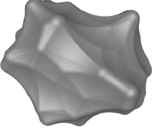
Figure 8: The molecular surface (alpha-hull) for crambin at probe-sphere radii (alpha value) of 10 ˚Angstroms.

face is recomputed from the beginning, although one could conceivably store the feasible cell description with each atom. Assuming the atoms of the molecule move along continuous trajectories, it should be possible to compute such surfaces (and indeed

-hulls and

-shapes) incrementally and efficiently by using the information from previous time steps.

Acknowledgments

8

References

[1] F. Aurenhammer. Power diagrams: Properties, algorithms and applications. SIAM Journal of Computing, 16(1):78–96, 1987.

[2] M. L. Connolly. Analytical molecular surface calculation. Journal of Applied Crystallography, 16:548–558, 1983.

[3] H. Edelsbrunner. Weighted alpha shapes. Technical Report UIUCDCS-R-92-1740, Department of Computer Science, University of Illinois at Urbana-Champaign, 1992.

[4] H. Edelsbrunner, D. G. Kirkpatrick, and R. Seidel. On the shape of a set of points in the plane. IEEE Transactions on Information Theory, IT-29(4):551– 559, 1983.

[5] H. Edelsbrunner and E. P. M¨ucke. Three-dimensional alpha shapes. ACM Transactions on Graphics, 13(1), 1994.

[6] I. Emiris and J. Canny. An efficient approach to removing geometric degenera-cies. In Eighth Annual Symposium on Computational Geometry, pages 74–82, Berlin, Germany, June 1992. ACM Press.

[7] F. M. Richards. Areas, volumes, packing and protein structure. Ann. Rev. Biophys. Bioengg., 6:151–176, 1977.

[8] R. Seidel. Linear programming and convex hulls made easy. In Sixth An-nual ACM Symposium on Computational Geometry, pages 211–215, Berke-ley, California, June 1990. ACM Press.

[9] A. Varshney and F. P. Brooks, Jr. Fast analytical computation of Richards’s smooth molecular surface. In G. M. Nielson and D. Bergeron, editors, IEEE Visualization ’93 Proceedings, pages 300–307, October 1993.