Classification of EMG Signals using Empirical
Mode Decomposition
Soona Shabani
Biomedical Group, CSE&IT Dept., Faculty of ECE, Shiraz
University, Shiraz, Iran.
Hossein Parsaei
EMG Lab., Waterloo University, Waterloo, Canada
Afshin Shaabany
fars telecommunication company, shiraz,iran
ABSTRACT
Discrimination of rehabilitation diseases based on electromyogram (EMG) signals is a hot topic among the biomedical society. Although many attempts have been made to obtain the informative features from the recorded EMG signals, specialists have still not satisfied with the achieved results. Therefore, this paper is aimed at introducing an effective way to enhance the classification rate among the three groups including: myopathy, neuropathy, and control simulated subjects. In this way, first, the empirical mode decomposition (EMD) is applied to the simulated signals in order to decompose each signal to its natural components. The resulted decomposed signal is used to classify these three groups. The achieved comparison results between the suggested method and other conventional method exhibit the superiority of our method in terms of classification accuracy among these groups. In addition, applying the paired T-test on the results supports the significance of our evolution (P<0.05).
Keywords
Classification, Electromyogram (EMG), Empirical Mode Decomposition (EMD).
1.
INTRODUCTION
Several neuromuscular disorders that affect the spiral cord, nerves, or muscles are existed. Neuromuscular pains has a high prevalence in various groups of people including young and old professionals in sport fields, older house wives, traditional artists who involve with making handcraft objects, young and elder labors, typists, etc. Early detection and diagnosis of such diseases is crucial for managing of their treatments [1].
Specialists diagnose the neuromuscular diseases using visual inspection of the recorded Electromyogram (EMG) of the patients and compare their shape and key points to the standard ones. Regarding the limitation of human eyes, it is obvious that visual template matching cannot be as accurate as the quantitative measures that automatically analyze all details of the recorded signals in time, frequency, and state-space domains.
EMG signals are naturally constructed by spatio-temporal integration of motor unit action potentials (MUAPs) which are activated in different depths and length [2]. EMG signals are easily caught from the forearm skin while to record each MUAP signal, a needle electrode is required to invade inside the muscle (beside a neuromuscular junction) the subject is asked to slightly contract that muscle. Electrical activity of a single anatomical motor unit (MUAP) represents the superposition of action potentials related to the muscle fibers within the recording range of the electrodes [3]. In other words, the aim is decomposing the EMG into MUAP patterns, because existence of each abnormality in the EMG signal is
originated by deterioration of MUAPs’ shape. These characteristic changes can be utilized to classify various types of neuromuscular diseases [4-6]. Hence, for detection and classification of each abnormality, first, EMG signals should be decomposed to its essential elements (by decomposing the signal into its natural subspaces) and then abnormality detection should be performed on decomposed subspaces.
The classification problem is mostly divided into three stages including; feature extraction, dimensionality reduction, and pattern classification. Several features can be extracted from EMGs in different domains such time, frequency, and state space.
Specialists in practice just use time domain features like duration (latency), amplitude, and phases of MUAPs that is still their gold-standard criteria due to the interpretation simplicity and its capability to differentiate myopathy from neuropathy diseases [7]. However, with increasing muscle force, the number of activated MUAPs recruited at higher firing rates incline; therefore, making it difficult for the neurophysiologist to distinguish the individual MUAP waveforms. In practice, specialists assess MUAPs’ shape in the screen and listen to their audio characteristics. As a result, an experienced specialist can detect abnormalities with a reasonable accuracy. Nevertheless, subjective MUAP assessment, although satisfactory for the detection of unequivocal abnormalities, may not be sufficient to describe less obvious deviations or mixed patterns of abnormalities [8].
An efficient way to over the practitioners’ shortcomings is to decompose EMG signal and then elicit informative features from different domains, and finally classify them into similar groups that present significant information for the assessment of neuromuscular pathology [1]. Several methods have been proposed to decompose EMG signals quantitatively. Buchthal et al. [9] developed one of the earliest methods for EMG decomposition, at which MUAPs were recorded photographically and finally were selected for analysis. Stalberg et al. [8] used waveform template matching and employed different shape parameters as input to a template matching technique. Stashuk and Qu [10] proposed a method in order to identify MUAPs based on power spectrum matching. Chauvet et al. [11] introduced a method allowing decomposition of EMG signals based on fuzzy logic techniques. All of these techniques deal only with MUAP detection and EMG decomposition, but they do not classify them according to their pathology.
subspace. Finally, support vector machine (SVM) classifier [15-17] is exploited to classify the extracted features.
The rest of this paper is structured as follows. In Section 2, the methods which are used in this study are explained in detail. Section 3, presents the experimental results produced by applying the simulated data to the methods described in the former part. Finally, the paper is concluded and future outline of this research is briefly described as future work.
2.
METHODS & MATERIALS
In this Section, first the proposed method is explained, and then one conventional method which implemented in this study is briefly described. Next, the characteristics of simulated data are described. Afterward, the evaluation criteria are explained.
2.1.proposed method
In this part, our proposed method is described which include three stages as depicted in Figure 1. First, the data is
segmented with window length of 0.5s (2000 samples). Then, signals are decomposed by empirical mode decomposition scheme into its essential subspaces.
In this decomposition scheme, different part of signal may have different extracted component. Therefore, we consider the same number of EMG components for all segments. In order to equalize the feature vector length, the segment with minimum number of base components is found. If this minimum number of components is indicated by M, only the first M segment components of all other windowed signals consider in the feature selection phase and the others are discarded. Next step is to extract features by Sequential Forward Selection strategy (SFS) [18] as discussed in section 2.4. Finally, these features are fed to support vector machine (SVM) classifier [15] to determine the classification rate among the three groups including: myopathy, neuropathy, and control simulated subjects.
2.2.emprical mode decomposition(EMD)
This decomposition method determines the intrinsic oscillatory modes within a data using its time scales characteristic and then decomposes the data accordingly. EMD is based on three assumptions: 1) the signal has at least two extrema with at least one maximum and one minimum; 2) the time scale characteristic is determined by the time lapse between the extrema; and 3) if the data does not have any extrema, but contains inflection points, then it can be differentiated once or more times to reveal the extrema.
According to Drazin [19], the first step in this procedure is to examine the data by eye. After that, one can identify the different scales directly in two ways: by the time lapse between the successive zero crossings, and by the time lapse between the successive alternations of local maxima and minima. The interlaced local extrema and zero crossings make a complicated data with one undulation is riding on top of another, and they, in turn, are riding on other undulations, and so on. These undulations explain various characteristic scales of data.
The purpose of EMD procedure is decomposing time series into superposition of components, with well-defined instantaneous frequency, which is called Intrinsic Mode Functions (IMF). An IMF is a function which satisfies two conditions: 1) in the whole data set, the number of extrema and the number of zero crossings must be either equal or differ at most by one; 2) at any point, the mean value of the envelope defined by the local maxima and one defined by the local minima is zero
.
The procedure of EMD Method which decomposes the signal f is as follows (n = 0 and f0= f):
Set h0= fn and k= 0.
Construct the Upper (Lower) Envelope for hk by
identifying all the local extrema and fitting all the
local maxima (minima) by a cubic spline interpolation to use as the upper/lower envelope denoted by Uk / Lk.
The mean value of U and L is determined (mk(t)) ,
and the kth component is defined as
k k
k
h
m
h
1
. If hk+1 is not an IMF, then increment k, return to
Step 2 and repeat the procedure (with hk+1 in place
of hk). Otherwise, define the nth IMF as cn=hk+1 and
the residual fn+1= fn–c1 which is essentially a slowly
varying portion of the signal. If a convergence criterion is not met, increment n and return to Step 1. Several convergence criterions have been proposed [13, 20, and 21]. In this work, a method with the aim of guaranteeing globally small fluctuations in the mean while taking into account local large excursions is applied to our data [20]. This method considers 2 thresholds θ1 and θ2
.
In this way, sifting is iterated until σ (t) < θ1: for a
prescribed fraction which defined as (1 − α) of the total duration, and also, σ (t) < θ2 for the remaining
fraction. α = 0.05, θ1 = 0.05, and θ2 = 10 θ1 are used
in this paper.
|
/
=|
k kk
m
a
2
/
)
(
k kk
U
L
a
This procedure called the sifting process, and after stopping, we obtain the following result:
n n
i
i
r
h
f
[image:2.595.50.521.278.315.2]1
Figure 1: Stages of determining the proposed feature
EMD Decomposition One segment of
EMG signal
Considering First M
Component Feature Extraction
However, as noted in [21, 22], intermittency and mode mixing are major problems to the use this decomposition on many signals. The situation can be improved by using a masking function as proposed in [23]. In this method, the first IMF component (h1) is used to describe the highest frequency
component of the signal. Then, after the Hilbert decomposition [20, 24] of h1 into a1 and f1, an energy
weighted mean is computed which gives the mean frequency of k samples:
ki k
i
i
f
i
a
i
f
i
a
f
1
1 1 1
2 1 1 _
)
(
)
(
)
(
)
(
Choosing the following masking signal can result in a good performance:
)
/
2
sin(
)
(
_ 0
f
n
f
sa
n
s
Choosing a0 can affect the performance of the algorithm.
Generally the optimal choice of that depends on the amplitudes and frequencies of the components, but 1.6 above the average amplitude of the components can be considered as a good value.
Thus, a decomposition of the data is obtained containing n empirical modes and a residue denoted as rn. The decomposed
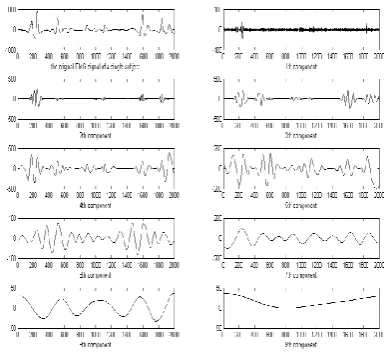
[image:3.595.77.272.489.667.2]components have several characteristic; they include different frequency bands ranging from high in the first base component to low in the last decomposed component. Moreover, these components are almost orthogonal, and in most cases, the leakage is too small. The result of applying the EMD decomposition process on one portion of simulated EMG data is shown in Figure 2. This data segment contains 9 IMFs and as can be seen the frequency of these IMFs is reduced from first to last component.
Figure 2: An EMG trial along with its decomposed IMF components, are depicted. The frequency of these IMFs is
reduced from up to down corresponding the first decomposition level to the last one.
2.3.The future extraction strategy
The purpose of feature extraction in this study is to extract a set of features that effectively distinguish the simulated EMG for myopathy, neuropathy, and control individuals. These features are quantitative representative of the EMG signals belong to each group, that finally applied to the classifier to be labeled. Therefore, In order to reduce the feature dimensionality that normally lead to decrease the classification time, and also improve the generalization, SFS is used in this paper which contains following steps:
1. Start with an empty feature set F0= {}.
2. Select the best feature x+ by the following criterion:
)]
(
[
max
arg
J
F
x
x
kF x k
3. Update Fk+1=Fk + x +
, k=k+1. 4. Go to 2
In this work, J is the mutual information [25], and the procedure will be continued until a decrease or an insignificance increase of J.
2.4.conventional compared method
To compare the proposed method to the state-of-art methodologies, one approach is considered and implemented here [26]. In this method Fast Fourier Transform (FFT) which represents the EMG contents into the frequency domain in terms of Fourier coefficients was used. Due to the high dimensionality of these coefficients, Principle Component Analysis (PCA) [27] was deployed to simultaneously preserving the EMG information and highly reducing the dimensionality of these features.
2.5.support vector machine
SVM has been developed based on the theory of structural risk minimization [15]. In a binary classification problem, the decision function of SVM is defined as follows:
𝑓 𝑥 =< 𝑤, ∅ 𝑥 > +𝑏
Where
<. , . >
denotes the dot product, and∅ 𝑥
is a kernel function mapping the input space to a higher dimensional feature space with probably more separability. In optimization heart of SVM, two objectives are considered: the first one is minimizing the margin width to preserve the locality and risk minimization, as far as margin width is inversely related to W; consequently, inverse of W should be minimized while the classification error should be minimized. Power two is considered for the variable w in order to construct a convex optimization function. By solving the following objective function, both of the mentioned objectives are satisfied. The optimum values of𝑏
and𝑤
can be obtained by taking two derivations from two variables of b and w.minimize: 𝑔 𝑤, 𝜉
𝑖=
1
2
| 𝑤 |
2+ 𝑐 𝜉
𝑖𝑁
𝑖=1
subject to: 𝑦
𝑖< 𝑤, ∅ 𝑥
𝑖> +𝑏 ≥ 1 − 𝜉
𝑖, 𝜉
𝑖≥ 0
minimize: 𝑊 ∝
= − ∝
𝑖𝑁
𝑖=1
+
1
2
𝑦
𝑖𝑦
𝑗𝑁
𝑗 =1 𝑁
𝑖=1
∝
𝑖∝
𝑗𝑘(𝑥
𝑖, 𝑥
𝑗)
subject to: ∝
𝑖𝑦
𝑖= 0, ∀𝑖: 0 ≤∝
𝑖≤ 𝑐
Ni=1
Where
∝
𝑖 is a Lagrange multiplier which corresponds to each sample𝑥
𝑖, and𝑘(𝑥
𝑖, 𝑥
𝑗)
is a kernel function that implicitly maps the input vectors into a suitable feature space:𝑘 𝑥
𝑖, 𝑥
𝑗=< ∅ 𝑥
𝑖), ∅(𝑥
𝑗>
In SVM, first, all samples are nonlinearly mapped into an implicitly higher dimensional space, and then, an optimal separating hyper-plane is estimated by the support vectors. The generalization performance of SVM is mainly affected by the kernel parameters and also, the regularization parameter c.
2.6.evaluation criteria
To validate the results, leave-one (patient)-out cross validation was employed in which accuracy (AC), specificity (SP) and sensitivity (SE) are calculated at each fold, and the average of these measurements were determined. In each experiment, according to leave-one-out cross validation, the train portion of data (features of all subjects except one) was fed to support vector machine and features of the out-patient in the training phase, is used as the test set. This process repeated for up to the number of subjects.
2.7.simulating EMG signals
In this section, the method for constructing the EMG signals for each group of subjects is explained. For each group 10 subjects were considered and to simulate their corresponding EMGs, statistical and morphological properties of each group were incorporated through the construction process of the signals. Sampling rate of the each simulated signal was set to 4000 sample per sec. It should be pointed out that EMG signals were simulated in the EMG laboratory of Waterloo University by the software of professor Stashuk.
3.
Experimental Results & Discussion
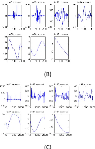
In this section, the results of applying the proposed scheme and also the explained compared method are presented. In the first experiment, we applied the EMD decomposition method to each segment. The result of applying this method on one segment of three normal, myopathy, and neuropathy groups of EMG signals can be seen in Figure 2. The results of applying this procedure to other segments of EMG data were similar to these figures depicted in Figure 3.(A)
(B)
[image:4.595.65.272.73.206.2](C)
Figure 3: the result of applying EMD procedure to EMG data A. subject with myopathy disorder B. subject with
myopathy disorder C. control subject.
As shown in Figure 3, there are several differences between the components of these groups. Therefore, we can employ the resulting components in the classification task.
In the second experiment, the EMD components were use as features. We decomposed signals with and without the masking signal explained in section 2.2. As shown in Table 1 and 2, these components can differentiate these groups from each other quite accurately. However, using masking signal improved the results as can be seen in Table 2.
Table 1: Results of applying EMD components to SVM (without masking function)
Classifier AC SP SE
[image:4.595.346.510.74.331.2]SVM 82.35 82.04 82.68
Table 2: Results of applying EMD components to SVM (wit masking function)
Classifier AC SP SE
SVM 87.96 85.22 90.7
[image:4.595.74.245.669.749.2]decreased with an insignificant decrease in the classification rate.
Table 3: Results of the proposed feature on the SVM classifier
classifier AC SP SE
SVM 86.82 85.04 88.62
Moreover, the result of applying the method, which was discussed in section 2.5 and proposed by Guler et al. [25], is shown in Tables 4.
Table 4: Results of applying the method proposed by Guler et al.
classifier AC SP SE
SVM 76.67 78.33 75.83
As it can be seen in Tables 3 and 4, the proposed scheme outperforms the compared methods. Using paired T-test analyses, this was found that this improvement is statistically significant (P<0.05). Hence, these features can discriminate these groups efficiently. In other words, in this work, EMD
was utilized to extract indicative feature. EMD forms a complete and nearly orthogonal basis for the signal. Therefore, the resulted IMFs are sufficient to describe the data. Additionally, as the signal is decomposed in time domain and with the same length of original data, we can observe varying frequencies at time. As experimental results suggests this decomposition reveals discriminative information which is hidden in the original data. IMFs of different subjects with different types don’t have the same structures. Hence, the extracted features could differentiate these classes almost accurately and also we can have a small feature dimension.
4.
CONCLUSION & FUTURE WORK
In this study, the empirical mode decomposition was used to classify three groups including: myopathy, neuropathy, and control simulated subjects. The results suggest that the proposed features might be a useful tool in the classification of these groups. Also, experimental results show that the resulted IMF components in different groups have different characteristics. In the future work, the results could be further investigated with a real data set and other features related to the structure of IMFs.
5.
REFERENCES
[1] Christodoulou, C. I.; Pattichis, C. S.: unsupervised pattern classification for the classification of EMG signals, IEEE Transactions on Biomedical Engineering, 46, 169-178 (1999).
[2] Butchal, F.: An Introduction to EMG, Copenhagen, Gyldendal (1957).
[3] Pattichis, C. S. ; Elia, A. G. Autoregressive and cepstral analyses of motor unit action potentials, Med. Eng. Phys., 21, 405-419 (1999).
[4] DeLuca C.J.: Towards understanding the EMG signal, 4th ed., Baltimore: Williams & Wilkinson (1978).
[5] Krarup C.: Pitfalls in electro diagnosis, J Neurophysiol, 81, 1115-1126 (1999).
[6] McGill K.C.: Optimal resolution of superimposed action potentials, IEEE Trans Biomed Engg. 49, 640-650 (2002).
[7] Pattichis, C.S.; Pattichis, M.S.: Time-Scale Analysis of Motor Unit Action Potentials, IEEE Transactions on Biomedical Engineering, 46, 325-329 (1999).
[8] Stalberg, E.; Andreassen, S,; Falck, B.; Lang, H.; Rosenfalck, A. Trojaborg, W.: Quantitative analysis of individual motor unit potentials: a proposition for standardized terminology and criteria for measurement, Journal of Clinical Neurophysiology, 3, 313-348 (1986).
[9] Buchthal, F.; Guld, C.; Rosenfalck, P.: Action Potential Parameters in Normal Human Muscle and their Dependence on physical variables, Acta Physiol Scand, 2, 200–218 (1954).
[10] Stashuk, D.; Bruin, H.D.: Automatic decomposition of selective needle-detected my electric signals, IEEE Trans Biomed Eng, 35, 1–10 (1988).
[12] Chauvet, E.; Fokapu, O.; Hogrel, J.Y.; Gamet, D.; Duchêne, J.: Automatic identification of motor unit action potential trains from electromyographic signals using fuzzy techniques, Med. Biol. Eng. Comput., 41, 646–653 (2003).
[13] Huang, N.E.; Shen, Z.; Long, S.R.; Wu, M.L.; Shih, H.H.; Zheng, Q.; Yen, N.C.; Tung, C.C.; Liu, H.H.: The empirical mode decomposition and Hilbert spectrum for nonlinear and nonstationary time series analysi, Proc. Roy. Soc.London A., 454, 903–995 (1998).
[14] Souza Neto, E.P.; Custaud, M.A.; Cejka, C.J.; Abry, P.; Frutoso, J.; Gharib C.; Flandrin, P.: Assessment of cardiovascular autonomic control by the Empirical Mode Decomposition, 4th Int. Workshop on Biosignal Interpretation, Como (I), 123-126 (2002).
[15] Wu, Z.; Schneider, E.K.; Hu Z.Z.; Cao, L.: The impact of global warming on ENSO variability in climate records, COLA Technical Report, 110 (2001).
[16] Vapnik, V. : Statistical Learning Theory, Wiley, New York (1998).
[17] Cai, Y.; Liu, X.; Xu, X.: Prediction of protein structural classes by support vector machines, Comput. Chemi.,26, 293-296 (2002).
[18] Reunanen, J.: Search Strategies. Feature Extraction Foundations and Applications Stud-Fuzz, 207, 119–136 2006.
[19] Drazin, P.G.: Nonlinear systems, Cambridge University Press (1992).
[20] Rilling, G.; Flandrin P.; Gonçalves P.: On Empirical Mode Decomposition and its algorithms, IEEE-EURASIP Workshop on Nonlinear Signal and Image Processing NSIP-03, Grado (I) (2003).
[22] Huang, N. E.; Shen, Z.; Long, S.: A New View of Nonlinear Water Waves: The Hilbert Spectrum, Annu. Rev. Fluid Mech., 31, 417–457 (1999).
[23] Deering R.; Kaiser, J.F.: The use of a masking signal to improve empirical mode decomposition, ICASSP (2005).
[24] Flandrin, P.; Rilling, G.; Gonc¸ P.: Empirical mode decomposition as a filter bank, IEEE Sig. Proc. Lett., 11, 112–114 (2004).
[25] Torkkola, K.: Information-Theoretic Methods, Feature Extraction Foundations and Applications StudFuzz, 207, 167–185 (2006).
[25] Nihal F.G.; Sabri, J.F.: Classification of EMG Signals Using PCA and FFT, Journal of Medical Systems, 29, 241-250 (2005).