R E S E A R C H
Open Access
Some algorithms for classes of split
feasibility problems involving paramonotone
equilibria and convex optimization
Q.L. Dong
1, X.H. Li
1, D. Kitkuan
2, Y.J. Cho
3,4and P. Kumam
2,5**Correspondence:
2KMUTTFixed Point Research
Laboratory, Department of Mathematics, Faculty of Science, King Mongkut’s University of Technology Thonburi (KMUTT), Bangkok, Thailand
5Department of Medical Research,
China Medical University Hospital, China Medical University, Taichung, Taiwan
Full list of author information is available at the end of the article
Abstract
In this paper, we first introduce a new algorithm which involves projecting each iteration to solve a split feasibility problem with paramonotone equilibria and using unconstrained convex optimization. The strong convergence of the proposed algorithm is presented. Second, we also revisit this split feasibility problem and replace the unconstrained convex optimization by a constrained convex optimization. We introduce some algorithms for two different types of objective function of the constrained convex optimization and prove some strong
convergence results of the proposed algorithms. Third, we apply our algorithms for finding an equilibrium point with minimal environmental cost for a model in electricity production. Finally, we give some numerical results to illustrate the effectiveness and advantages of the proposed algorithms.
MSC: 47H05; 47H07; 47H10; 54H25
Keywords: Split feasibility problem; Equilibria; Constrained convex optimization; Practical model
1 Introduction and the problem statement
LetH1andH2be two real Hilbert spaces with inner product·,·and reduced norm · ,
CandQbe nonempty closed convex subsets inH1andH2, respectively.
In [7], Censor and Elving first introduced thesplit feasibility problem(shortly, SFP) in Euclidean space, which is formulated as follows:
Findx∗∈Csuch thatAx∗∈Q,
whereA:H1→H2is a bounded linear operator. The SFP can be a model for many inverse
problems where constraints are imposed on the solutions in the domain of the linear op-erator as well as in its range. It has a variety of specific applications in real world such as medical care, image reconstruction and signal processing (see [5,14–17,21,38,39] for more details).
Letf :C×C→Rbe a bifunction such thatf(x,x) = 0 for allx∈C. Theequilibrium problem(shortly, EP)
Findx∗∈Csuch thatfx∗,y≥0 for ally∈C
was firstly introduced by Fan [19] and further studied by Blum and Oettli [2]. The solution set of the EP is denoted bySol(EP). The EP is a generalization of many mathematical mod-els, including variational inequality, fixed point, optimization, complementarity problems (see, for instance, [2,4,13,18,20,22,23,25,31,33–36]).
Recently, Yen et al. [37] investigated the followingsplit feasibility probleminvolving paramonotone equilibria and convex optimization (shortly, SEO):
Problem 1.1 Findx∗∈Csuch thatf(x∗,y)≥0 for ally∈Candg(Ax∗)≤g(z) for allz∈ H2,
wheregis a proper lower semi-continuous convex function onH2. Also, they introduced
the following algorithm to solve Problem1.1:
Algorithm 1.1 For anyxk∈C, takeηk∈∂k
2 f(xk,xk) and define
αk=
βk
γk
,
whereγk=max{δk,ηk}. Compute
yk=PC
xk–αkηk
.
Take
μk:=
⎧ ⎨ ⎩
0, if∇h(yk) = 0,
ρk h(y k)
∇h(yk)2, if∇h(yk)= 0,
and compute
zk=PC
yk–μkA∗(I–proxλg)
Ayk.
Let
xk+1=akxk+ (1 –ak)zk.
In Algorithm1.1,proxλgdenotes proximal mapping of the convex functiongwithλ> 0, and the parameters{ak},{δk},{βk},{k}and{ρk}are taken as in Algorithm3.1(see below
Sect.3).
Note that Algorithm1.1involves two exact projections onto the feasible setC, which limits the applicability of the method, especially when such projections are hard to com-pute. It is well known that only in a few specific instances the projection onto a convex set has an explicit formula. When the feasible setCis a general closed convex set, we must solve a nontrivial quadratic problem in order to compute the projection ontoC.
The paper is organized as follows: Sect.2deals with some definitions and lemmas for the main results in this paper. In Sect.3, we introduce a new algorithm, which involves a projection in each iteration. In Sect.4, we introduce two algorithms and study their convergence. In Sect.5, we provide a practical model for an electricity market and some computational results for the model.
2 Preliminaries
The following definitions and lemmas are useful for the validity and convergence of the algorithms.
Definition 2.1 LetHbe a Hilbert space,T:H→Hbe a mapping and letK⊆H. (i) Tis said to benonexpansiveif
Tx–Ty ≤ x–y
for allx,y∈H.
(ii) Tis said to befirmly nonexpansiveif
Tx–Ty ≤ x–y,Tx–Ty
for allx,y∈H, or
0≤Tx–Ty, (I–T)x– (I–T)y
for allx,y∈H.
(iii) Tis said to beLipschitz continuouswith Lipschitz constantLif
Tx–Ty ≤Lx–y
for allx,y∈H.
(iv) Tis said to beα-averagedif
T= (1 –α)I+αS,
whereα∈(0, 1)andS:H→His a nonexpansive mapping.
Lemma 2.1([1, Proposition 4.4]) Let H be a Hilbert space and T:H→H be a mapping. Then the following are equivalent:
(i) T is firmly nonexpansive; (ii) I–Tis firmly nonexpansive.
Lemma 2.2([3,9]) The composition of finitely many averaged mappings is averaged.In particular,if T1isα1-averaged and T2isα2-averaged,whereα1,α2∈(0, 1),then the
com-position T1T2isα-averaged,whereα=α1+α2–α1α2.
For a mappingT:H→H,Fix(T) denotes the set of fixed points ofT, i.e.,
Fix(T) :={x∈H:Tx=x}.
It is well known that every nonexpansive operatorT :H→Hsatisfies the following in-equality:
(x–Tx) – (y–Ty),Ty–Tx≤1
2 (x–Tx) – (y–Ty)
2
for allx,y∈Hand so
x–Tx,y–Tx ≤1
2x–Tx
2
for allx∈Handy∈Fix(T) (see, for example, [11, Theorem 3], [12, Theorem 1]). LetHbe a real Hilbert space andKbe a nonempty convex closed subset ofH. For each pointx∈H, there exists a unique nearest point inK, denoted byPK(x), such that
x–PK(x) ≤ x–y
for ally∈K. The mappingPK:H→Kis calledthe metric projectionofHontoK. It is well
known thatPK is a nonexpansive mapping ofHontoK and even a firmly nonexpansive
mapping. So,PKis also12-averaged, which is captured in the following lemma:
Lemma 2.3 For any x,y∈H and z∈K,the following hold: (i) PK(x) –PK(y)2≤ x–y;
(ii) PK(x) –z2≤ x–z2–PK(x) –x2.
Some characterizations of the metric projectionPK are given by the two properties in
the following lemma:
Lemma 2.4 Let x∈H and z∈K.Then z=PK(x)if and only if PK(x)∈K and
x–PK(x),PK(x) –y
≥0
for all x∈H and y∈K.
Lemma 2.5 Let C be a nonempty closed convex subset in a Hilbert space H and PC(x)be
the metric projection of x onto C.Then we have
(i) x–y,PC(x) –PC(y) ≥ PC(x) –PC(y)2for allx,y∈C;
(ii) zk–yk ≤β k.
Lemma 2.6 Let {vk} and{δ
k} be the nonnegative sequences of real numbers satisfying
vk+1≤vk+δ
kwith
∞
k=1δk< +∞.Then the sequence{vk}is convergent.
Lemma 2.7 Let H be a real Hilbert space,{ak}be a sequence of real numbers such that
0 <a<ak<b< 1for all k≥1and{vk},{wk}be the sequences in H such that
lim sup
k→+∞
vk ≤c, lim sup k→+∞
and,for some c> 0,
lim sup
k→+∞
akvk+
1 –akwk =c.
Thenlimk→+∞vk–wk= 0.
Definition 2.2([28]) Thenormal coneofKatv∈K, denote byNK, is defined as follows:
NK(v) :=
d∈H:d,y–v ≤0,∀y∈K.
Definition 2.3([1, Definition 16.1]) Thesubdifferential setof a convex functioncat a pointxis defined as follows:
∂c(x) :=ξ∈H:c(y)≥c(x) +ξ,y–x,∀y∈H.
Define byιKtheindicator functionof the setK, i.e.,
ιK(x) =
⎧ ⎨ ⎩
0 x∈K,
+∞ otherwise.
It is well known that∂ιK(x) =NK(x) and (I+λNK)–1=PK for anyλ> 0.
Letf :H×H→Rbe a bifunction. We need the following assumptions onf(x,y) for our algorithms and convergence:
(A1) For eachx∈C,f(x,x) = 0 andf(x,·) is lower semi-continuous and convex onC; (A2)∂2f(x,x) is nonempty for any> 0 andx∈Cand is bounded on any bounded subset ofC, where∂2f(x,x) denotes-subdifferential of the convex functionf(x,·) atx, that is,
∂2f(x,x) :=η∈H1:η,y–x+f(x,x)≤f(x,y) +,∀y∈C
; (1)
(A3) f is pseudo-monotone on C with respect to every solution of the EP, that is, f(x,x∗)≤0 for anyx∈C,x∗∈Sol(EP) andf satisfies the following condition, which is called thepara-monotonicity property:
x∗∈Sol(EP), y∈C, fx∗,y=fy,x∗= 0 ⇒ y∈Sol(EP);
(A4) For allx∈K,f(·,x) is weakly upper semi-continuous onC.
3 A new algorithm for Problem1.1and its convergence analysis
In this section we give a new algorithm for Problem1.1and analyze its convergence. Recall that the proximal mapping of the convex functiongwithλ> 0, denoted byproxλg, is defined as the unique solution of the strongly convex programming problem:
proxλg(u) =argmin
v∈H2
g(v) + 1
2λv–u
2
. (P(u))
The proximal mapping has some good properties, namely, it is firmly nonexpansive and
For anyλ> 0, we set
h(x) :=1
2 (I–proxλg)Ax
2
.
By using the necessary and sufficient optimality condition for convex programming, we can see thath(x) = 0 if and only ifAxsolvesP(u) withu=Ax. Note that, even thoughg may not be differentiable,his always differentiable and∇h(x) =A∗(I–proxλg)Ax(see, for example, [28]).
Algorithm 3.1 Take positive parametersδ,ξand the real sequences{ak},{δk},{βk},{k},
{ρk}satisfying the following conditions: for eachk∈N,
0 <a≤ak≤b< 1, 0 <ξ≤ρk≤4 –ξ,
δk>δ> 0, βk> 0, k≥0,
lim
k→+∞ak= 1 2, ∞
k=1
βk
δk
= +∞, ∞
k=1
βk2= +∞, ∞
k=1
βkk
δk
< +∞.
Step1. Choosex1∈Cand letk:= 1.
Step k. Havexk∈Cand take
μk:=
⎧ ⎨ ⎩
0 if∇h(xk) = 0,
ρk h(x k)
∇h(xk)2 if∇h(xk)= 0,
then compute
yk=xk–μkA∗(I–proxλg)Axk.
Takeηk∈∂
k
2 f(yk,yk) and define
αk=
βk
γk
,
whereγk=max{δk,ηk}. Compute
zk=PC
yk–αkηk
. (2)
Let
xk+1=akxk+ (1 –ak)zk.
Lemma 3.1([24]) Let S be the set of solutions of Problem1.1and y∈S.If∇h(xk)= 0,then
yk–y 2≤ xk–y 2–ρk(1 –ρk)
h2(xk)
∇h(xk)2.
Lemma 3.2([29]) For each k≥1,the following inequalities hold: (i) αkηk ≤βk;
(ii) zk–yk ≤β k.
Lemma 3.3 Let y∈S.Then,for each k≥1such that∇h(xk)= 0,we have
xk+1–y 2≤ xk–y 2– (1 –ak)ρk(4 –ρk)
h2(xk)
∇h(xk)2
+ 2(1 –ak)αkf
yk,y+Ak,
and,for each k≥1such that∇h(xk) = 0,we have
xk+1–y 2≤ xk–y 2+ 2(1 –ak)αkf
yk,y+Ak,
where Ak= 2(1 –ak)(αkk+βk2).
Proof By the definition ofxk+1, we have
xk+1–y 2= akxk+ (1 –ak)zk–y 2
≤ak xk–y 2
+ (1 –ak) zk–y 2
. (3)
Moreover, we have
zk–y 2= y–yk+yk–zk 2
= yk–y 2– yk–zk 2+ 2yk–zk,y–zk
≤ yk–y 2+ 2yk–zk,y–zk.
Since it follows from Lemma2.4and (2) that
zk–yk+αkηk,x–zk
≥0
for allx∈C, by takingx=y, we obtain
zk–yk+αkηk,y–zk
≥0 ⇐⇒ αkηk,y–zk
≥yk–zk,y–zk
and hence
zk–y 2≤ yk–y 2+ 2α
kηk,y–zk
= yk–y 2+ 2αkηk,y–yk
+ 2αkηk,yk–zk
It follows fromηk∈∂
k
2 f(yk,yk) that
fyk,y–fyk,yk
≥ηk,y–yk
–k ⇐⇒ f
yk,y+k≥
ηk,y–yk
. (5)
On the other hand, from Lemma3.2(ii), it follows that
αkηk,yk–zk
≤αkηk yk–zk ≤βk2.
From (4), (5) andαk> 0, it follows that
zk–y 2≤ yk–y 2+ 2α kf
yk,y+ 2α
kk+ 2βk2. (6)
Now, we consider two cases:
Case1. If∇h(xk)= 0, then, thanks to Lemma3.1, we have
yk–y 2= xk–y 2–ρk(4 –ρk)
h2(xk)
∇h(xk)2.
Combining this inequality with (3) and (6), we obtain xk+1–y 2≤ xk–y 2+ 2(1 –ak)αkf
yk,y
– (1 –ak)ρk(4 –ρk)
h2(x k)
∇h(xk)2
+Ak,
whereAk= 2(1 –ak)(αkk+βk2).
Case2. If∇h(yk) = 0, then, by the definition ofyk, we can writeyk=xk. Now, by the same
argument as in Case 1, we have
zk–y 2≤ yk–y 2+ 2αkf
yk,y+ 2αkk+ 2βk2.
Then we have
xk+1–y 2≤ xk–y 2+ 2(1 –ak)αkf
yk,y+Ak,
whereAk= 2(1 –ak)(αkk+βk2). This completes the proof.
Theorem 3.1 Suppose that Problem 1.1 admits a solution. Then, under Assumptions (A1)–(A4),the sequence{xk}generated by Algorithm3.1strongly converges to a solution
of Problem1.1.
Proof Claim1. The sequence{xk–y2}is convergent for ally∈S. Indeed, lety∈S. Since
y∈Sol(EP) andf is pseudomonotone onCwith respect to every solution of (EP), we have
If∇h(xk)= 0, then, since
ρk(4 –ρk)
h2(xk)
∇h(xk)2≥
0,
it follows from Lemma3.3that xk+1–y 2≤ xk–y 2+Ak,
whereAk= 2(1 –ak)(αkk+βk2). Sinceαk=βγkk withγk=max{δk,ηk},
+∞
k=1
αkk= +∞ k=1 βk γk k≤ +∞ k=1 βk δk
k< +∞.
Note that+k∞=1βk2< +∞and 0 <a<ak<b< 1 and so we have
+∞
k=1
Ak< 2(1 –a) +∞
k=1
αkk+βk2
< +∞.
Now, using Lemma2.6, we see that{xk–y2}is convergent for ally∈S. Hence the
se-quence{xk}is bounded. Then, by Lemma3.2, we can see that{yk}is bounded too.
Claim2.lim supk→∞f(yk,y) = 0 for ally∈S. By Lemma3.3, for eachk≥1, we have
–2(1 –ak)αkf
yk,y≤ xk–y 2– xk+1–y 2+Ak.
Summing up both sides in the above inequality, we obtain
∞
k=1
–2(1 –ak)αkf
yk,y< +∞.
On the other hand, using Assumption (A2) and the fact that{xk}is bounded, we see that
{ηk}is bounded. Then there existsL>δsuch thatηk ≤Lfor eachk≥1. Therefore,
we have
γk
δk
=max
1,ηk
δ+k
≤L
δ
and hence
αk=
βk
γk ≥
δ
L
βk
δk
.
Sinceyis a solution, by pseudomonotonicity off, we have –f(yk,y)≥0, which together
with 0 <a<ak<b< 1 implies
∞
k=1
(1 –b)βk
δk
But, from∞k=1βk
δk = +∞, it follows that
lim sup
k→+∞ f
yk,y= 0
for ally∈S.
Claim3. For anyy∈S, suppose that{ykj}is the subsequence of{yk}such that
lim sup
k→+∞
fyk,y= lim
j→+∞f
ykj,y (7)
andy∗is a weakly cluster point of{ykj}. Theny∗belongs toSol(EP).
Without loss of generality, we can assume that{ykj}weakly converges toy∗asj→ ∞. Sincef(·,y) is upper semi-continuous, by Claim 2, we have
fy∗,y≥lim sup
j→+∞
fykj,y= 0.
Sincey∈Sandf is pseudomonotone, we havef(y∗,y)≤0 and sof(y∗,y) = 0. Again, by pseudomonotonicity off,f(y,y∗)≤0 and hencef(y∗,y) =f(y,y∗) = 0. Then, by paramono-tonicity (Assumption (A3)), we can conclude thaty∗is also a solution of (EP).
Claim 4. Every weakly cluster pointx¯ of the sequence {xk}satisfies x¯∈K andAx¯ ∈
argming. Letx¯be a weakly cluster point of{xk}and{xkj}be a subsequence of{xk}weakly converging tox¯. Thenx¯∈K. From Lemma3.3, if∇h(xk)= 0, then we have
(1 –ak)ρk(4 –ρk)
h2(xk)
∇h(xk)2 ≤ x
k–z 2– xk+1–z 2+A k.
If∇h(xk) = 0, then we have
0≤ xk–z 2– xk+1–z 2+Ak.
LetN1:={k:∇h(xk)= 0}. Summing up, we can write
k∈N1
(1 –ak)ρk(4 –ρk)
h2(xk)
∇h(xk)2 ≤ x
0–z 2+
∞
k=1
Ak< +∞.
Combining this fact with the assumptionξ≤ρk≤4 –ξ(for someξ > 0) and 0 <a<ak<
b< 1, we can conclude that
k∈N1
h2(xk)
∇h(xk)2< +∞.
Moreover, since∇his Lipschitz continuous with constant A2, we see that∇h(xk)2
is bounded. So,h(xk)→0 ask∈N
1andk→ ∞. Note thath(xk) = 0 fork∈/N1.
Conse-quently, we have
lim
k→+∞h
By the lower semi-continuity ofh,
0≤h(x¯)≤lim inf
j→+∞ h
xkj= lim
k→+∞h
xk= 0,
which implies thatAx¯is a fixed point of the proximal mapping ofg. ThusAx¯is a minimizer ofg. From (8) and the fact that∇h(xk)2is bounded, it follows that
lim
k→+∞μk= 0,
which yields
lim
k→+∞
yk–xk = lim
k→+∞μk
A∗(I–proxλg)Axk = 0.
Thus{ykj}weakly converges tox¯.
Claim5.limk→+∞xk=limk→+∞yk=limk→+∞P(xk) =x∗, where x∗ is a weakly cluster point of the sequence satisfying (7). From Claims 3 and 4, we can deduce thatx∗belongs toS. By Claim 1, we can assume that
lim
k→+∞ x
k–x∗ =c< +∞.
By Lemma3.2, we have
zk–x∗ ≤ yk–x∗ + zk–yk
≤ xk–x∗ + xk–yk +βk,
which implies that
lim sup
k→+∞
zk–x∗ ≤lim sup
k→+∞
xk–x∗ + xk–yk +β k
=c.
On the other hand, we have
lim
k→+∞
ak
xk–x∗+ (1 –ak)
zk–x∗ = lim
k→+∞
xk+1–x∗ =c.
By applying Lemma2.7withvk:=xk–x∗,wk:=zk–x∗, we obtain
lim
k→+∞
zk–xk = 0.
Employing arguments, similar to those used in the proof of Theorem 1 in [37], we have
lim
k→+∞x
k=x∗.
4 Algorithms and convergence analysis
In [37], Yen et al. presented an application of Problem1.1to a model of electricity produc-tion, in whichzdenotes the quantity of the materials andg(z) is the total environmental fee that companies have to pay for environmental pollution while using materialszfor production. So, fromx∈C, it follows thatz=Ax∈ {z:z=Ax,x∈C}.
However, in actual production, since the resources are limited, there are usually stricter constraints on the quantity of the materials such asz∈Q, whereQis a nonempty closed convex set ofH2. Therefore, it is necessary to replace the unconstrained convex
optimiza-tion problemminx∈H2g(x) with theconstrained convex optimizationas follows:
min
x∈Qg(x), (9)
whose solution is denoted bySol(Q,g). By using (9), Problem1.1becomes the following problem:
Problem 4.1 Find x∗∈C such that f(x∗,y)≥0 for all y∈C such that Ax∗∈Q and g(Ax∗)≤g(z) for all z∈Q,
whose solution is denoted by
Γ :=Γ(C,Q,f,g,A) :=z∈Sol(EP) :Az∈Sol(Q,g).
Throughout this paper, we assumeΓ =∅.
In this section, we discuss two cases that the function g is differentiable or non-differentiable. The corresponding algorithms and their convergence are provided next.
4.1 The case whengis differentiable
We need to make the following assumption on the mappingg: (B)gisL-Lipschitz differentiable withL> 0, i.e.,
∇g(x) –∇g(y) ≤Lx–y
for allx,y∈H2.
It is easy to verify that the constrained convex optimization problem (9) is equivalent to the followingvariational inequality problem:
∇gz∗,z–z∗≥0 for allz∈Q, (10)
and the variational inequality problem (10) is equivalent to the followingfixed point prob-lem:
z∗=PQ(I–ν∇g)z∗, (11)
Firstly, define two functions
h(x) := I–PQ(I–ν∇g)
Ax 2 (12)
and
l(x) := A∗I–PQ(I–ν∇g)
Ax 2,
whereν∈(0,2L).
Algorithm 4.1 Take the real sequences{ak},{δk},{βk},{k}and{ρk}as in Algorithm3.1.
Step1. Choosex1∈Cand letk:= 1. Step k. Havexk∈Cand take
μk:=
⎧ ⎨ ⎩
0 ifl(xk) = 0,
ρkh(x k)
l(xk) ifl(xk)= 0,
then compute
yk=xk–μkA∗
I–PQ(I–ν∇g)
Axk. (13)
Takeηk∈∂
k
2 f(yk,yk) and define
αk=
βk
γk
,
whereγk=max{δk,ηk}. Compute
zk=PC
yk–αkηk
.
Let
xk+1=akxk+ (1 –ak)zk.
Now, we need the following lemmas to prove the convergence of Algorithm4.1:
Lemma 4.1([8, Lemma 6.2]) Assume that a mapping g:H2→H2satisfies Assumption
(B)andν∈(0,2L).Let y∈Γ.Ifl(xk) = 0,then it follows that
yk–y 2≤ xk–y 2–ρ
k(1 –ρk)
h2(xk)
l(xk) .
Proof LetT=PQ(I–ν∇g). Sincey∈Γ, it follows from (11) thatAyis a fixed point of
T. From the proof of [32, Theorem 4.1], it follows thatT is 2+4νL-averaged and so it is nonexpansive. By (13) and Lemma2.3(i), we have
– 2μk
xk–y,A∗(I–T)Axk. (14)
By the nonexpansivity ofTand (2), we have
xk–y,A∗(I–T)Axk
=Axk–y, (I–T)Axk
=Axk–y– (I–T)Axk+ (I–T)Axk, (I–T)Axk
=TAxk–Ay,Axk–TAxk+ (I–T)Axk 2
≥1
2 (I–T)
Axk 2. (15)
Combining (14) and (15) and using the definitions ofh(x) andl(x), we obtain yk–y 2≤ xk–y 2+μ2klxk–μkh
xk
= xk–y 2–ρk(1 –ρk)
h2(xk)
l(xk) .
This completes the proof.
Remark4.1 From (15), it follows thatl(x) = 0 impliesh(x) = 0.
Using Lemma4.1and following the lines of the proof of Lemma3.3, we have the follow-ing:
Lemma 4.2 Let y∈Γ.Then,for each k≥1such that l(xk)= 0,we have
xk+1–y 2≤ xk–y 2–ρk(1 –ρk)
h2(xk) l(xk)
+ 2(1 –ak)αkf
yk,y+Ak
and,for each k≥1such that l(xk) = 0,we have
xk+1–y 2≤ xk–y 2+ 2(1 –ak)αkf
yk,y+Ak,
where Ak= (1 –ak)(αkk+βk2).
Next we establish the convergence of Algorithm4.1.
Theorem 4.1 Under Assumptions(A1)–(A4)and(B),the sequence{xk}generated by Al-gorithm4.1strongly converges to a solution of Problem4.1.
4.2 The case whengis non-differentiable
Letg:Q→R∪ {+∞}be a proper convex lower semi-continuous function. Denote by
gλ(z) :=min
u∈Q
g(u) + 1 2λu–y
2
(16)
theMoreau–Yosida approximateof the functiongwith the parameterλ. It is easy to see that the solution of (16) converges to that ofminx∈Qg(x) asλ→ ∞.
For the mapping defined in (16), we have following result.
Lemma 4.3 The constrained optimization problem
min
x∈Qgλ(x) (17)
is equivalent to the fixed point formulation
x∗=PQ
x∗–ν(I–proxλg)x∗, (18)
whereν∈(0, +∞).
Proof It is well known that problem (17) is equivalent to the following problem:
min
x∈H2
ιQ(x) +gλ(x)
. (19)
Note that the differentiability of the Yosida-approximategλ(see, for instance, [28]) secures the additivity of the subdifferentials, and so we can write
∂ιQ(x) +gλ(x)
=∂ιQ(x) +
I–proxλg
λ (x).
The optimality condition of (19) can be then written as follows:
0∈λ∂ιQ(x) + (I–proxλg)(x), (20)
where the subdifferential ofιC atxisNC(x). The inclusion (20) in turn yields (18). This
completes the proof.
Set
h(x) = I–PQ
I–ν(I–proxλg)Ax 2
and
l(x) = A∗I–PQ
I–ν(I–proxλg)Ax 2.
Algorithm 4.2 Take the real sequences{ak},{δk},{βk},{k}and{ρk}as in Algorithm3.1.
Take a positive parameterν.
Step1. Choosex1∈Cand letk:= 1. Step k. Havexk∈Cand take
μk:=
⎧ ⎨ ⎩
0 ifl(xk) = 0,
ρkh(x k)
l(xk) ifl(xk)= 0,
then compute
yk=xk–μk
A∗I–PQ
I–ν(I–proxλg)Axk. (21)
Takeηk∈∂
k
2 f(yk,yk) and define
αk=
βk
γk
,
whereγk=max{δk,ηk}. Compute
zk=PC
yk–αkηk
.
Let
xk+1=akxk+ (1 –ak)zk.
Remark4.2 Letν= 1 in Algorithm4.2, then formula (21) becomes
yk=xk–μk
A∗(I–PQ◦proxλg)
Axk,
which yields
yk=xk–μkA∗(I–proxλg)
Axk,
whenQ=H2. So, Algorithm3.1is a special case of Algorithm4.2.
We need the following lemmas for the proof of the convergence of Algorithm4.2.
Lemma 4.4 Letν∈(0, 1].Then operator PQ(I–ν(I–proxλg))is nonexpansive.
Proof By the fact thatproxλg is firmly nonexpansive and Lemma2.1,I–proxλgandν(I–
proxλg) are also firmly nonexpansive. So, using Lemma2.1again,I–ν(I–proxλg) is firmly nonexpansive. Thus, from Lemma2.2, it follows thatPQ(I–ν(I–proxλg)) is34-averaged
and hence nonexpansive. This completes the proof.
Theorem 4.2 Letν∈(0, 1].Then,under Assumptions(A1)–(A4),the sequence{xk}
gen-erated by Algorithm4.2strongly converges to a solution of Problem4.1.
The proof of Theorem4.2is similar to that of Theorem3.1, so here we omit it.
One thing to note about proof of Theorem4.2is that fromh(x¯) = 0 it follows thatAx¯is a fixed point ofPQ(I–ν(I–proxλg)). Thus, by Lemma4.3,Ax¯is a solution of (17).
5 Numerical examples
In this section, we provide two numerical examples to compare different algorithms. All programs are written in Matlab version 7.0 and performed on a desktop PC with Intel(R) Core(TM) i5-4200U CPU @ 2.30 GHz, RAM 4.00 GB.
Example5.1 First, we consider an equilibrium-optimization model which was investi-gated by Yen et al. [37]. This model can be regarded as an extension of a Nash–Cournot oligopolistic equilibrium model in electricity markets. The latter model has been investi-gated in some research papers (see, for example, [10,27]).
In this equilibrium model, it is assumed that there arencompanies. Letxdenote the vector whose entryxistands for the power generated by companyi. Following Contreras
et al. [10], we suppose that the pricepi(s) is a decreasing affine function ofswiths=
n i=1xi,
that is,
pi(s) =α–βis.
Then the profit made by companyiis given by
fi(x) =pi(s)xi–ci(xi),
whereci(xi) is the cost for generatingxiby the companyi.
Suppose thatCiis the strategy set of companyi, that is, conditionxi∈Cimust be
satis-fied for eachi. Then the strategy set of the model isC:=C1×C2× · · · ×Cn.
Actually, each company seeks to maximize its profit by choosing the corresponding pro-duction level under the presumption that the propro-duction of the other companies are para-metric input. A commonly used approach to this model is based upon the famous Nash equilibrium concept.
Now, we recall that a pointx∗∈C=C1×C2× · · · ×Cnis anequilibrium pointof the
model if
fi
x∗≥fi
x∗[xi]
for allxi∈Ciandi= 1, 2, . . . ,n, wherex∗[xi] stands for the vector obtained fromx∗ by
replacingx∗i withxi. By taking
f(x,y) :=Ψ(x,y) –Ψ(x,x)
with
Ψ(x,y) := –
n
i=1
fi
x[yi]
the problem of finding a Nash equilibrium point of the model can be formulated as follows:
Findx∗∈Csuch thatfx∗,x≥0 for allx∈C. (EP)
In [37], Yen et al. extended this equilibrium model by additionally assuming that the companies use some materials to produce electricity.
Letal,idenote the quantity of materiall(l= 1, . . . ,m) for producing one unit of electricity
by companyi(i= 1, . . . ,n). LetAbe the matrix whose entries areal,i. Then entrylof the
vectorAxis the quantity of materiallfor producingx. Using materials for production may cause environmental pollution, for which companies have to pay a fee. Suppose thatg(Ax) is the total environmental fee for producingx.
The task now is to find a productionx∗ such that it is a Nash equilibrium point with a minimum environmental fee, while the quantity of the materials satisfies constraintQ. This problem can be formulated as thesplit feasibility problemof the following form:
Findx∗∈Csuch thatfx∗,x≥0 for allx∈C
andgAx∗≤g(Ax) for allAx∈Q. (SEP)
Suppose that, for everyi, costcifor production and environmental feegare increasing
convex functions. The convexity assumption here means that both the cost and fee for producing a unit of product increase as the quantity of the product gets larger.
Under this convexity assumption, it is not hard to see (see also Quoc et al. [27]) that problem (EP) withf given by (22) can be formulated as follows:
Findx∗∈Csuch thatfx∗,x:=B˜1x∗–a¯,x–x∗
+ϕ(x) –ϕx∗≥0 for allx∈C, (23)
where
¯
a:= (α,α, . . . ,α)T,
B1:=
⎛ ⎜ ⎜ ⎜ ⎜ ⎝
b1 0 0 . . . 0
0 b2 0 . . . 0
..
. ... ... . .. ... 0 0 0 . . . bn
⎞ ⎟ ⎟ ⎟ ⎟
⎠, B˜1:= ⎛ ⎜ ⎜ ⎜ ⎜ ⎝
0 b1 b1 . . . b1
b2 0 b2 . . . b2
..
. ... ... . .. ... bn bn bn . . . 0
⎞ ⎟ ⎟ ⎟ ⎟ ⎠,
ϕ(x) :=xTB1x+ n
i=1
ci(xi).
(24)
Note that, whenciis differentiable and convex for eachi, problem (23) is equivalent to
the followingvariational inequality problem:
Findx∗∈Csuch thatB˜1x∗–a¯+∇ϕ
x∗,x–x∗≥0 for allx∈C.
We tested the proposed algorithm with the cost function given by
ci(xi) =
1 2pix
2
wherepi≥0. In [37], Yen et al. showed that functionf(x,y) defined by (23), (24) and (25)
satisfies Assumptions (A1), (A2) and (A4).
In [37], the author denoted byg(z) the total environmental fee. It is unreasonable. Firstly, the total environmental fee should be included in the cost, that is, it is a part ofci(xi).
Secondly, it is supposed that the companies behave as players in an oligopolistic market, but at the same time they are subordinated to the centralized planning decision in order to minimize the total environmental fee for the whole system. That is, the model is not concordant with the real system behavior.
It may be reasonable to denote byg(z) the restriction for the emission of contaminants. To protect the environment, governments generally adopt policies to restrict emissions of contaminants.
Assume that the production of electricity bringspcontaminants and governments re-quire that the quantity of contaminants brought by the production of one unit of electricity is in a given region. We use a setK⊂Rpto denote this region.
Letbk,ldenote the quantity of the contaminantk(k= 1, . . . ,p) for consuming one unit of
materiall(l= 1, . . . ,m). LetBbe the matrix whose entries arebk,l. Then entrykof vector
Bzis the quantity of contaminantkfor consuming one unit of materialzl(l= 1, . . . ,m). So,
the quantity of contaminantk(k= 1, . . . ,p) for producing one unit of electricity is entryk ofBAx, andBAxshould be in the setK, i.e.,BAx∈K. We getBz∈Kwhen lettingz=Ax.
Therefore we define functiong(z) as follows:
g(z) = 1
2 Bz–PK(Bz)
2
, (26)
which is differentiable and∇g(z) =BT(I–P
K)(Bz) (see, e.g., [6]).
Take the sequences{βk},{k},{δk}of the parameters as follows:
βk=
4
k+ 1, k= 0, δk= 3, γk=max
3,ηk
for eachk≥1 and takeν=1.99B. The entries of matrixAwere randomly generated in the interval [0, 5]. In the bifunctionf(x,y) defined by (23), (24) and (25), the parametersα= 0.5 andbi,piandqifor eachi= 1, . . . ,nwere generated randomly in the interval (0, 1], [1, 3],
and [1, 3], respectively. In the functiong(z), we takeB∈Rp×Rm, and its elements are
generated randomly in (0, 1).
Since functiong(z) is differentiable, we use Algorithm4.1to solve Problem4.1and com-pare it with Algorithms1.1and3.1. In Algorithms1.1and3.1we substituteproxλg with I–ν∇gand do not consider the constraint setQ.
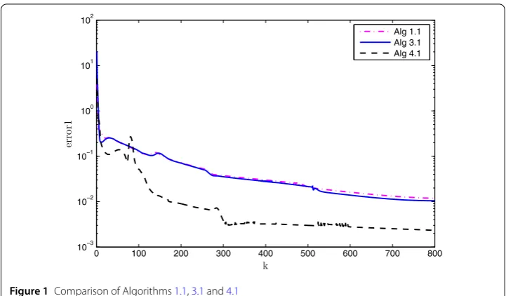
The computational results are shown in Figs.1and2. The horizontal and vertical axes show iterationk, as well as error1(k) :=xk–xk–1and error2(k) :=Axk–P
Q(Ayk),
re-spectively. We solve the model withm= 15 and taken= 10 as the number of companies. From Figs.1and2, we have two conclusions as follows:
(a) The “error1” of Algorithm4.1is smaller than that of Algorithms1.1and3.1and the “error1” of Algorithm3.1is slightly smaller than that of Algorithm1.1.
Figure 1Comparison of Algorithms1.1,3.1and4.1
Figure 2Comparison of Algorithms1.1,3.1and4.1
Next we give a numerical procedure in an infinite-dimensional space and compare Al-gorithm4.1with a numerical algorithm which is based on the Halpern modification of [8, Algorithm 6.1] as follows:
Algorithm 5.1
xk+1=τkx1+ (1 –τk)U
xk+γA∗(T–I)Axk,
whereT:=PQ(I–λ∇g),U:=PC(I–λf), andγ ∈(0, 1/L),Lis the spectral radius of the
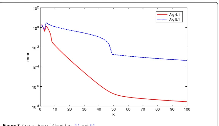
Figure 3Comparison of Algorithms4.1and5.1
According to the condition of the convergence of Halpern-type algorithm, we assume thatlimk→∞τk= 0 and
∞
k=1τk=∞.
Example5.2 Suppose thatH=L2([0, 1]) with normx:= (01|x(t)|2dt)12 and inner
prod-uctx,y:=01x(t)y(t)dt,x,y∈H. LetC:={x∈H:x ≤1}be the unit ball,Q:={x∈H:
x(t),sin(10x(t)) ≤1}. Define an operatorF:C→Hby
F(x)(t) = 1
0
x(t) –B(t,s)px(s)ds+q(t)
for allx∈Candt∈[0, 1], where
B(t,s) = 2tse
t+s
e√e2– 1, p(x) =cosx, q(t) =
2tet
e√e2– 1.
As shown in [30],F is monotone andL-Lipschitz-continuous withL= 2. Letf(x(t), y(t)) =Fx(t),y(t) –x(t),g(x)(t) =12x(t)2and (Ax)(t) = 3x(t) for allx∈H.
Letx1(t) = 1. Take the sequences{α
k},{βk},{k},{δk}of the parameters as follows:
αk=
1
2, βk= 4
k+ 1, k= 0, δk= 3, γk=max
3,ηk
for eachk≥1 and takeν= 1.99Lg . We take λ= 1 according to the numerical tests since the constants of the inverse strong monotonicity of∇gandf are unknown. Takeτk=k1+1
andγ =ρ(0.9A∗A) for Algorithm5.1. We useerror=12PC(xk) –xk2+12PQ(Axk) –Axk2to
measure the error of thekth iteration.
Numerical results are given in Fig.3, which illustrate that Algorithm4.1behaves better than Algorithm5.1.
6 Conclusions
constraint to the minimization problem of the total environmental fee. Two algorithms are introduced to approximate the solution and their strong convergence is analyzed.
Acknowledgements
We sincerely thank Prof. S. He for his helpful discussion and the reviewers for their valuable suggestions and useful comments that have led to the present improved version of the original manuscript.
Funding
The first author was supported by the scientific research project of Tianjin Municipal Education Commission (No. 2018KJ253). The fifth author was supported by the Theoretical and Computational Science (TaCS) Center under Computational and Applied Science for Smart Innovation Cluster (CLASSIC), Faculty of Science, KMUTT. The authors acknowledge the financial support provided by King Mongkut’s University of Technology Thonburi through the “KMUTT 55th Anniversary Commemorative Fund”. Furthermore, Poom Kumam was supported by he Thailand Research Fund (TRF) and the King Mongkut’s University of Technology Thonburi (KMUTT) under the TRF Research Scholar Award (Grant No. RSA6080047).
Availability of data and materials
Data sharing not applicable to this article as no datasets were generated during the current study.
Competing interests
The authors declare that they have no competing interests.
Authors’ contributions
All authors contributed equally to the writing of this paper. All authors read and approved the final manuscript.
Author details
1Tianjin Key Laboratory for Advanced Signal Processing, College of Science, Civil Aviation University of China, Tianjin,
P.R. China.2KMUTTFixed Point Research Laboratory, Department of Mathematics, Faculty of Science, King Mongkut’s
University of Technology Thonburi (KMUTT), Bangkok, Thailand.3Department of Mathematics Education, Gyeongsang
National University, Jinju, Korea. 4School of Mathematical Sciences, University of Electronic Science and Technology of
China, Chengdu, P.R. China. 5Department of Medical Research, China Medical University Hospital, China Medical
University, Taichung, Taiwan.
Publisher’s Note
Springer Nature remains neutral with regard to jurisdictional claims in published maps and institutional affiliations.
Received: 17 December 2018 Accepted: 18 March 2019
References
1. Bauschke, H.H., Combettes, P.L.: Convex Analysis and Monotone Operator Theory in Hilbert Spaces. Springer, Berlin (2011)
2. Blum, E., Oettli, W.: From optimization and variational inequalities to equilibrium problems. Math. Stud.63, 123–145 (1994)
3. Byrne, C.: A unified treatment of some iterative algorithms in signal processing and image reconstruction. Inverse Probl.20, 103–120 (2004)
4. Ceng, L.C.: Approximation of common solutions of a split inclusion problem and a fixed-point problem. J. Appl. Numer. Optim.1, 1–12 (2019)
5. Censor, Y., Bortfeld, T., Martin, B., Trofimov, A.: A unified approach for inversion problems in intensity modulated radiation therapy. Phys. Med. Biol.51, 2353–2365 (2006)
6. Censor, Y., Elfving, T., Kopf, N., Bortfeld, T.: The multiple-sets split feasibility problem and its applications for inverse problems. Inverse Probl.21, 2071–2084 (2005)
7. Censor, Y., Elving, T.: A multiprojections algorithm using Bregman projections in a product spaces. Numer. Algorithms 8, 221–239 (1994)
8. Censor, Y., Gibali, A., Reich, S.: Algorithms for the split variational inequality problem. Numer. Algorithms59, 301–323 (2012)
9. Combettes, P.L.: Solving monotone inclusions via compositions of nonexpansive averaged operators. Optimization 53, 475–504 (2004)
10. Contreras, J., Klusch, M., Krawczyk, J.B.: Numerical solution to Nash–Cournot equilibria in coupled constraint electricity markets. IEEE Trans. Power Syst.19, 195–206 (2004)
11. Crombez, G.: A geometrical look at iterative methods for operators with fixed points. Numer. Funct. Anal. Optim.26, 157–175 (2005)
12. Crombez, G.: A hierarchical presentation of operators with fixed points on Hilbert spaces. Numer. Funct. Anal. Optim. 27, 259–277 (2006)
13. Dong, Q.L., Cho, Y.J., Zhong, L.L., Rassias, T.M.: Inertial projection and contraction algorithms for variational inequalities. J. Glob. Optim.70, 687–704 (2018)
14. Dong, Q.L., He, S., Zhao, J.: Solving the split equality problem without prior knowledge of operator norms. Optimization64, 1887–1906 (2015)
16. Dong, Q.L., Tang, Y.C., Cho, Y.J., Rassias, T.M.: “Optimal” choice of the step length of the projection and contraction methods for solving the split feasibility problem. J. Glob. Optim.71, 341–360 (2018)
17. Dong, Q.L., Yao, Y., He, S.: Weak convergence theorems of the modified relaxed projection algorithms for the split feasibility problem in Hilbert spaces. Optim. Lett.8, 1031–1046 (2014)
18. Dong, Q.L., Yuan, H.B., Cho, Y.J., Rassias, T.M.: Modified inertial Mann algorithm and inertial CQ-algorithm for nonexpansive mappings. Optim. Lett.12, 87–102 (2018)
19. Fan, K.: Fixed point and minimax theorems in locally convex topological linear spaces. Proc. Natl. Acad. Sci. USA38, 121–126 (1952)
20. He, S.N., Tian, H.L.: Selective projection methods for solving a class of variational inequalities. Numer. Algorithms80, 617–634 (2019)
21. He, S.N., Tian, H.L., Xu, H.K.: The selective projection method for convex feasibility and split feasibility problems. J. Nonlinear Convex Anal.19, 1199–1215 (2018)
22. Konnov, I.V.: Combined Relaxation Methods for Variational Inequalities. Springer, Berlin (2000)
23. Konnov, I.V.: The method of pairwise variations with tolerances for linearly constrained optimization problems. J. Nonlinear Var. Anal.1, 25–41 (2017)
24. Moudafi, A., Thakur, B.S.: Solving proximal split feasibility problems without prior knowledge of operator norms. Optim. Lett.8, 2099–2110 (2014)
25. Muu, L.D., Oettli, W.: Convergence of an adaptive penalty scheme for finding constrained equilibria. Nonlinear Anal. 18, 1159–1166 (1992)
26. Parikh, N., Boyd, S.: Proximal algorithms. Found. Trends Optim.1, 123–231 (2013)
27. Quoc, T.D., Muu, L.D.: Iterative methods for solving monotone equilibrium problems via dual gap functions. Comput. Optim. Appl.51, 709–728 (2012)
28. Rockafellar, T.R., Wets, R.: Variational Analysis. Springer, Berlin (1998)
29. Santos, P., Scheimberg, S.: An inexact subgradient algorithm for equilibrium problems. Comput. Appl. Math.30, 91–107 (2011)
30. Shehu, Y., Dong, Q.L., Jiang, D.: Single projection method for pseudo-monotone variational inequality in Hilbert spaces. Optimization68, 385–409 (2019)
31. Xiao, Y.B., Huang, N.J., Cho, Y.J.: A class of generalized evolution variational inequalities in Banach spaces. Appl. Math. Lett.25, 914–920 (2012)
32. Xu, H.K.: Averaged mappings and the gradient-projection algorithm. J. Optim. Theory Appl.150, 360–378 (2011) 33. Yao, Y., Leng, L., Postolache, M., Zheng, X.: Mann-type iteration method for solving the split common fixed point
problem. J. Nonlinear Convex Anal.18, 875–882 (2017)
34. Yao, Y., Liou, Y.C., Yao, J.C.: Iterative algorithms for the split variational inequality and fixed point problems under nonlinear transformations. J. Nonlinear Sci. Appl.10, 843–854 (2017)
35. Yao, Y., Yao, J.C., Liou, Y.C., Postolache, M.: Iterative algorithms for split common fixed points of demicontractive operators without priori knowledge of operator norms. Carpath. J. Math.34, 459–466 (2018)
36. Yao, Y.H., Postolache, M., Liou, Y.C.: Strong convergence of a self-adaptive method for the split feasibility problem. Fixed Point Theory Appl.2013, Article ID 201 (2013)
37. Yen, L.H., Muu, L.D., Huyen, N.T.T.: An algorithm for a class of split feasibility problems: application to a model in electricity production. Math. Methods Oper. Res.84, 549–565 (2016)
38. Zhao, J.: Solving split equality fixed-point problem of quasi-nonexpansive mappings without prior knowledge of operators norms. Optimization64, 2619–2630 (2015)