Disk formation and structure
Carsten Dominik
1Anton Pannekoek Institute for Astronomy, University of Amsterdam, The Netherlands
Abstract.In this chapter, we cover the formation of protoplanetary disk as a natural by-product of the gravitational collapse of a slowly rotating, hydrostatic cloud. We also summarise the structure of such a disk as it results from hydrostatic equilibrium and viscous accretion.
1 Introduction
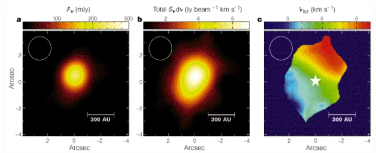
In this chapter we look at the basic processes disk formation and of disk structure. Why do disks form in the first place? How will matter be distributed, radially and vertically? We will focus mainly on the structure of disks resulting from viscous evolution. Another important process affecting disk structure is external irradiation. As this is so strongly coupled with the spectral energy distribution we observe from protoplanetary disks, we will cover this part in the chapter on spectral energy distributions. The original idea of a protosolar nebula dates back to Kant & Laplace in the 18th century who used the observed structure of the planetary system to propose the existence of a flattened structure around the Sun from which the planets formed, explaining both the flattened geometry and the aligned angular momenta of the Sun and the planetary orbits (nothing was known back then about planetary rotation). The confirmation that such disks indeed exist and that they are a common by-product of star formation dates back to the late 1980’s and early 1990’s, when the first mm images (Beckwith et al. 1986, Sargent & Beckwith 1987, Rodriguez et al. 1992) and spectroscopy (e.g. Koerner et al. 1993) of such disks were taken (Fig. 1). The mm dust emission revealed the extended structures around young stars and the double peaked line profiles were proof of the regular Keplerian rotation pattern. The launch of the Hubble Space Telescope in 1990 opened a new window for research on protoplanetary disks. The high spatial resolution from space enabled the detailed imaging of the Orion nebula, a star forming region at a distance of 450 pc (O’Dell et al. 1992). These images were taken with the Wide Field Camera in several optical narrow band Filters such as Hα, [Oiii], [Oi] and [Sii]. The data shows not only that such protoplanetary disks are ubiquitous around newly formed stars (50% of stars show disk detection), but reveals also the impact of disk irradiation and erosion by nearby hot O and B stars.
2 Disk formation as a result of the collapse of a rotating cloud
Protoplanetary disks are the natural byproduct of the formation of a star from a rotating cloud of gas. For the purpose of this chapter we are not concerned how exactly the details of the collapse process
First Lecture of the Summer School “Protoplanetary Disks: Theory and Modelling Meet Observations” DOI: 10.1051/
C
Owned by the authors, published by EDP Sciences, 2015 /201
epjconf 5 0 0 0 2
7KLVLVDQ2SHQ$FFHVVDUWLFOHGLVWULEXWHGXQGHUWKHWHUPVRIWKH&UHDWLYH&RPPRQV$WWULEXWLRQ/LFHQVHZKLFKSHUPLWV XQUHVWULFWHGXVHGLVWULEXWLRQDQGUHSURGXFWLRQLQDQ\PHGLXPSURYLGHGWKHRULJLQDOZRUNLVSURSHUO\FLWHG
Figure 1.In each panel, the full-width at half-maximum of the synthesised beam is shown at top left, and offsets in arcseconds from the stellar position are indicated along the vertical and horizontal axes. (a) Thermal continuum from dust grains, at wavelengthλ=1.3 mm. The flux density (F) scale is shown at the top of the panel. (b) CO(2-1) emission, integrated across the full velocity range (+2.4 to+7.6 km s−1) in which emission is measured above the 3σlevel. The scale at the top of the panel provides the integrated intensities (S dv). (c) Intensity-weighted mean gas velocities at each spatial point of the structure shown in b. The stellar (systemic) velocity,Vlsr ≈ 5.1 km s−1, is represented by green. Blue-shifted (approaching) and red-shifted (receding) velocity components are shown as blue and red, respectively. The star symbol indicates the position of MWC480. Reprinted by permission from Macmillan Publishers Ltd: Nature (Mannings et al. 1997), copyright (1997).
work - there are a number of competing theories that describe this phase. One of them is the inside-out collapse model (Shu 1977), but in other scenarios the entire cloud starts collapsing at the same time. What we will consider here is how the fact that a cloud is rotating ever so slowly before the collapse will lead to the formation of an accretion disk.
We assume that the cloud was in hydrostatic equilibrium for some time before collapse, and we will therefore assume that it rotates as a solid body. Also, we assume that the cloud rotates slowly, so that the centrifugal force is initially very small compared to the gravity and pressure forces at any point in the cloud. Then, the early stages of collapse are almost radial. In this limit, we can distinguish between an outer envelope which stays almost spherical and an inner region that gets distorted due to rotation and forms an equatorial accretion disk.
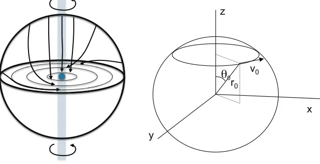
Depending on the specific angular momentum (that is the angular momentum per unit of mass) of a gas parcel, it will either be able to accrete onto the protostellar core (very low specific angular momentum) or accrete onto the equatorial disk at some radius corresponding to its angular momen-tum. A particle initially located on the rotation axis of the cloud has zero angular momentum and will simply fall directly to the center, i.e. the star. The maximum possible distance from the star at which such a gas parcel can end up is called the centrifugal radiusrc, and it is reached by particles that are
θ
0x
y
z
v0 r0
Figure 2. Sketch of a collapse including rotation. Left panel: A rotating cloud collapses, and different parcels fall according to their specific angular momentum along a path associated with their angular momentum. Right panel: Definition of the geometric quantities describing the initial position and velocity of the fluid element before falling.
approximate the orbit quite well by a parabola with focus at the center of the cloud. The distance from the star can then be written as a function of the true anomaly using Kepler’s equation for the parabola
r= req
1+cosΨ , (1)
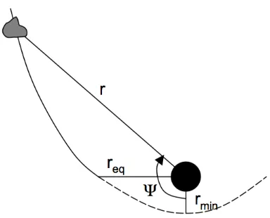
where the coordinates and quantities are introduced in Fig. 3. If the fluid element would reach the clos-est distancermin, the maximum orbital velocity would at that point be perpendicular to the direction
to the star and have the value
vmax=
2GM∗
rmin
, (2)
whereM∗is the mass of the protostar+disk. Note thatM∗may be a function of time during star formation, so fluid elements that fall early on experience a different gravitational potential than fluid elements that fall late.
The fluid element will never reach the minimum stellar distance though. Instead, it collides with the forming disk and with matter coming in on a similar trajectory from the other side of the midplane atΨ =π/2 (see Fig. 4). The specific angular momentum jis preserved along the entire curve and most easily computed at the theoretical minimum distance because radius vector and velocity are perpendicular. There we find
j=rminvmax=
2GM∗rmin . (3)
Since the fluid element reachesrminatΨ=0, Eq. (1) implies thatrmin=req/2. Therefore, we can write
the radius at which the fluid element reaches the midplane as
req=
j2
Figure 3. Sketch of a parabolic orbit in rotating infall. The sketch is in the orbital plane of the falling fluid element. A fluid element with polar coordinates (r,Ψ) falls in and hits the equatorial disk at a radiusreq. In the absence of the disk, the fluid element would have reached the smaller distancerminbefore swinging back out again.
Now we can express the specific angular momentum in terms of the initial quantitiesΩ0 (angular velocity) andθ0(inclination of orbital plane with respect to the rotation axis,θ0=90ois the midplane, see Fig. 2)
j=R2Ω
0sinθ0 , (5)
whereRis the distance from the center at which the fluid element starts its fall. We can see that fluid elements from larger distances will have larger specific angular momentum and will therefore become part of the disk at larger and larger distances from the star. In the Shu inside-out collapse (Shu 1977), that layer starts to fall when the rarefaction wave that starts in the center of the cloud att=0, reaches R, i.e. when it has travelled with the isothermal sound speedcsto that location. Then,R=cst, and we
can write
j=R2Ω0sinθ0=c2st2Ω0sinθ0 , (6)
The angular momentum is larger for higher values ofθ0and has a maximum atθ0=90o. Using the expression for the core mass as a function of timeMr(t)c3st/Gfrom Shu’s model (Shu 1977), we
can rewritereqas
req=cst3Ω20sinθ20 . (7)
Forθ0=90o,reqis maximal, and we call this value thecentrifugal radiusof the disk
rc=cst3Ω0≈7.33 AU
cs
0.35 km/s
Ω
10−14s−1
2
t 105yr
3
. (8)
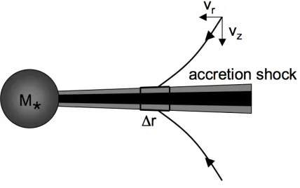
Figure 4.Schematic view of disk formation during the collapse of a rotating spherical cloud. Matter is falling toward the disk on mirrored path from locations above and below the midplane. The matter is stopped suddenly above the disk with an accretion shock that dissipated the free-fall energy.
Sect. 2 describes how a flat disk forms during the collapse of a rotating cloud. Since the simple collapse problem outlined there is spherically symmetric and the rotation itself axisymmetric, the trajectories of infalling material from the top are mirrored at the equatorial plane. The infalling fluid elements, which follow parabolic trajectories, thus collide in the equatorial plane with matter coming from the other side of the cloud. An accretion shock forms where the material collides and this accretion shock extends over the entire centrifugal radiusrc. If the excess heat energy from the shock can be efficiently radiated away, a thin disk structure forms in the equatorial plane (Fig. 4).
The disk is supported against gravity by its rotation, but also to a lesser extent by the gas pressure gradient. To first order we can thus approximate the orbital velocity of the gas by the Keplerian orbital speed
vK= ΩKr=
GM∗(t)
r . (9)
We callΩKthe Kepler frequency
ΩK=
GM∗(t)
r3 . (10)
At different stages of the evolution,M∗(t) may not yet be the full mass of the star.
In the shock and subsequent cooling process, the vertical component of the infalling velocity is dissipated, so that the material within the disk is left with the parallel component of its infalling veloc-ityvr(see Fig. 4). However, this remaining velocity is not necessarily equal to the Keplerian velocity
3 Disk structure
For deriving the general equations of disk structure, we follow the motion of an annulus of the disk and use the vertically integrated form in all equations, i.e. the surface densityΣinstead of the physical densityρgas. Matter can flow into the annulus and out of it with a velocityvr. This picture contains
the implicit assumption that vertical motions in the disk can be neglected (vz=0) and that the radial
motion is the same at all heights (vr(r,z)=vr(r)).
We consider in the following an axisymmetric disk and assume that the surface density can be written in the general form ofΣ(r,t), which is an integral of the mass densityρgas(r,z) over the disk heightz
Σ(r,t)=
∞
−∞ρgas(r,z) dz . (11)
Then the vertically integrated continuity equation reads as
r∂Σ ∂t +
∂
∂r(rΣvr)=0 (12)
and the vertically integrated conservation of orbital angular momentum becomes
r∂ ∂t
r2ΩΣ+ ∂ ∂r
r2Ω·rΣvr
= 1
2π ∂τ
∂r . (13)
The two velocity components arevr andvΦ=rΩ. The angular momentum of a thin annulus of the
disk is 2πrΔrΣr2Ω, whereΔris the width of the annulus. The term on the right hand side of Eq. (13) arises from the viscous torques in the disk.
We briefly revisit here the concept of torque. A force that acts on the mass center of a body will cause a straight motion. If the same force acts on a point offthe mass center, the body will start to rotate as well. The torqueτis then the product of the forceFand the lever, i.e. the distance from the mass centerr
τ=rFsinθ (14)
whereθis the angle between the force vector and the lever vector. The accretion disk is not rotating as a solid body and so we can apply the concept of torque on each annulus in the disk. The neighbouring annulus will exert a force on it proportional to the difference in orbital velocities, the orbital velocity gradient dΩ/dr. The force is called the shear force or viscous force.
The rate of shearing due to the orbital velocity gradient isrdΩ/dr. which has the units of s−1. Without describing yet the details of the viscosity or angular momentum transport, we note that
τ=2πr·νΣrdΩ
dr ·r=2πr 3νΣdΩ
dr . (15)
Here,νis the kinematic viscosity andτis the torque exerted on an annulus in the disk. It is the product of the circumference, the viscous force per unit length (νΣA=νΣrdΩ/dr) and the leverr.
Using the expression for the torqueτ, we can rewrite Eq. (13) as
∂ ∂t
r2ΩΣ+1 r
∂ ∂r
r2Ω·rΣvr =1 r ∂ ∂r νΣr3dΩ
dr
. (16)
We can now use the continuity equation (Eq. 12) to eliminate the time dependence and simplify this to
Σvr ∂(r2Ω)
∂r = 1 r
∂ ∂r
νΣr3dΩ
dr
The derivatives ofΩcan be worked out, if we assume that the orbital frequency equals the Kepler frequencyΩK. Then, this equation yields an expression for the radial velocity in the disk
vr=−
3
Σ√r ∂ ∂r
νΣ√r . (18)
Alternatively, we can insert Eq. (17) into Eq. (12) to eliminatevrand obtain
∂Σ
∂t = 1 r ∂ ∂r ⎡ ⎢⎢⎢⎢⎢ ⎣ d dr(r
2Ω)
−1 ∂
∂r
νΣr3
−dΩ
dr⎤⎥⎥⎥⎥⎥⎦ . (19)
If we assume again thatΩ = ΩK, we can simplify this to
∂Σ
∂t = 3 r ∂ ∂r √ r∂ ∂r
νΣ√r . (20)
3.1 Steady state disk structure
In steady state, the disk structure follows from radial and angular momentum conservation and the assumption that the vertical component of gravity from the star is balanced by the vertical gas pressure gradient (vertical hydrostatic equilibrium). We study for this a disk annulus at a distancerfrom the star. Material can flow into and out of the annulus with the velocityvrin radial direction. The radial
momentum conservation equation for a steady-state flow is
vr ∂vr
∂r − v2 φ r + 1 ρgas ∂P ∂r +
G M∗
r2 =0, (21)
wherevris the radial velocity of the gas,vφis the circular velocity, andM∗is the mass of the central star. The gas sound speed is defined asc2
s =∂P/∂ρgas, wherePis the gas pressure and ρgas is the gas density. For an ideal gas, cs =
k Tg/(μmp). Here, k is the Boltzmann constant, Tg is the
gas temperature,μis the mean molecular weight of the gas, and mp is the proton mass. The four terms in the above equation arise from radial mass flow, centrifugal force, gas pressure, and gravity. Since pressure typically decreases with increasing radius, the third term is nearly always negative; effectively, gas pressure resists the gravitational force, resulting in gas rotating at sub-Keplerian orbital velocities.
Following (Eq. 13), assuming steady-state (e.g. ∂/∂t=0) and using the expression for the torque τ, the angular momentum conservation equation becomes
∂ ∂r
rvrΣr2Ω
=∂∂
r
νΣr3dΩ dr
, (22)
where the left-hand side is the radial change in angular momentum and the right-hand side arises from the viscous torques. Integrating this equation yields the following expression
νΣdΩ
dr = ΣvrΩ + C
2πr3 . (23)
At the inner edge of the disk, the shear vanishes because the disk is truncated there. So at that point dΩ/dr=0. We can use this to get an expression for the integration constant
Here, ˙M=2πrΣ(−vr), because in an accretion flow, the radial velocity is inward and thus negative. For
simplicity, we assume that the disk extends down to the star. Then, the shear vanishes close to the star for
C=M˙GM∗R∗ . (25)
The integration constant can thus be seen as the influx of angular momentum through the disk. With this andΩ=ΩK=
GM∗/r3, the disk surface density becomes
Σ(r)= M˙ 3πν
⎛ ⎜⎜⎜⎜⎜
⎝1−
R∗ r
⎞ ⎟⎟⎟⎟⎟
⎠ , (26)
for radii much larger than the stellar radius. Note that the viscosityνis not a constant in the equation, but ˙Mobviously is.
3.2 Vertical disk structure
The vertical (z-direction) disk structure is found by solving the equation of hydrostatic equilibrium,
1 ρgas
∂P ∂z =
∂ ∂z
G M∗ √
r2+z2
. (27)
For an ideal gas, pressure and density are connected byP/ρgas=c2s=kT/(μmp), which can be used to
eliminateP. If the disk is vertically thin (zr) and the gas temperature does not depend onz(i.e. a vertically isothermal disk), Eq. (27) can be directly integrated to give the vertical density structure,
ρgas(r,z)=ρc(r) e−z 2/(2H2
gas), (28)
whereρc(r) is the density at the disk midplane and the gas scale height is given by
Hgas=
kTcr3/(μmpGM∗), (29)
whereTcis the midplane gas temperature. This equation shows that the gas scale height is the ratio
of the gas sound speed to the angular velocity (Hgas=cs/Ω). In reality, neitherTgnorμare constant
withz, and this can lead to large changes in the density structure high up in the disk. However, since we are here concerned with the mass dominating part of the disk close to the midplane, we work with these simplifying assumptions.
4 Radial disk structure
Having found an expression for the scale height, we return to the radial disk structure. We parametrise the viscosity asν=αcsHgas(which will be introduced later in Sect. 5.2 after a detailed discussion of the viscosity in disks). Inserting this relation along with Eq. (29) into Eq. (26), and assumingrR∗ we find
Σ = μmp
√ G M
3πk
˙ M αTcr3/2
. (30)
For a disk with a simple powerlaw midplane temperature profile,Tc ∝r−q, the surface density is
Further, the midplane density may be written as
ρc Σ/Hgas = ρin
r rin
3 2q−3
, (31)
whereρinis the density at the inner disk radiusrin. Assuming a simple powerlaw for the temperature profile is a first guess, but is there actually a way to determine the temperature profile within an accretion disk?
In an accretion disk, the energy generation is predominantly through viscous torques,τ(see also the discussion in the chapter on heating and cooling processes in disks, Woitke 2015). The net torque on a disk annulus with widthΔris equal to the difference between the torque on the outer and inner surface
τ(r+ Δr)−τ(r)= ∂τ
∂rΔr . (32)
The energy generated by this torque is then
Ω∂τ∂
rΔr=
∂
∂r(τΩ)−τ dΩ
dr
Δr . (33)
The first term, when added up over the entire disk, is simplyτΩ|rout−τΩ|rin and thus given by the
disk boundary conditions. The second term describes the local energy dissipation and thus the heat generation in an annulus in the disk. The energy generation per unit surface area is given by τ(dΩ/dr)Δr/(2πrΔr). We assume that this energy is not transported in the disk, but is radiated away locally through the two surfaces of the disk, withσT4
disk, whereTdisk is the effective temperature of the disk. Therefore we have (note the factor 2 due to the two sides of the disk)
σTdisk4 =−τdΩ/dr 4πr =−
1 2νΣ
rdΩ dr
2
=9
8νΣΩ
2 . (34)
Here we have filled in the torqueτusing Eq. (15). Also, we have assumed that the disk has a Keplerian rotation profileΩ = GM∗/r3. Using the relation found between the mass accretion rate and the viscosity, ˙M=3πνΣforrR∗, we can eliminate the viscosity from this equation
σTdisk4 = 3 8πM˙Ω
2 .
(35)
This yields a temperature profile of
Tdisk =
3 8πσM˙Ω
2
1/4
, (36)
thus ar−3/4 profile. We see that the disk temperature does not depend on the viscosity. The implicit assumption here is that the viscosity of the disk corresponds to its accretion rate, an observable quan-tity. Hence we do not need to know the details of the angular momentum transport to describe the disk structure. Using a relatively high observed accretion rate for a very young T Tauri star (M∗=1 M) of 10−7 M
5 Angular momentum transport
The specific angular momentum, which is the angular momentum per unit mass, stored in a 1 Mdisk with a size of 10 AU is 3×1053cm2/s. On the other hand, a 1 M
star rotating at break-up velocity has a specific angular momentum of 6×1051 cm2/s. Hence, the original angular momentum of the disk is 50 times higher than the maximum allowed for a star. Since angular momentum is strictly conserved, there needs to be a process that actually transports angular momentum away to prevent it from accumulating on the star. The main possibilities are a torque from the external medium (e.g. magnetic fields), viscosity inside the disk transporting angular momentum to the outer disk, and disk winds taking angular momentum away. In the following, we discuss the basic principle of angular momentum transport within the disk. Disks winds are certainly important as well, but their theory is complex and we ignore them in this course.
If we assume for a moment that the disk rotates with Keplerian speed and consider only two particles with massesm1andm2, we can write their total (kinetic plus potential) energyEand angular momentumJas
E=−GM∗ 2
m1 r1 +
m2 r2
(37)
J=m1vΦ,1r1+m2vΦ,2r2 (38)
= GM∗m1 √
r1+m2 √
r2
,
wherer1 andr2 are the corresponding distances of the two masses from the central star with mass M∗. From the conservation of angular momentum of the total system, it follows that a small change in orbit for one of the masses requires a corresponding change for the other one
∂J ∂r =−m1
1 2√r1
(39)
ΔJ= dJ dr1Δ
r1+ dJ dr2Δ
r2=0 (40)
m1Δ r1 √
r1 =− m2Δ
r2 √
r2
(41)
The same of course holds true if we consider two neighboring annuli in the disk.
This process requires a way of connecting the two particles (or rings of material) with each other. So, what remains to be identified is the source of this coupling. We can consider for example the friction between the two annuli to be caused by their difference in rotation speed (shear motion). However, since we deal here with a gas, diffusion plays a role in transporting gas in both directions, inward and outward. We can hence consider small turbulent random motions as a cause of radial mixing of material and thus as a cause of coupling the various annuli with the disk.
5.1 Turbulent viscosity
We can derive a simple estimate of the molecular viscosityνmthrough
νm≈λcs , (42)
whereλis the mean free path of the molecules given by 1/(nσm), the product of gas particle density
physical size of molecules (2×10⁻¹⁵ cm2), we obtain for a typical distance of 10 AU in the disk a molecular viscosity of
νm=
1 nσm
cs=
5×10⁴
1012×2×10−15 cm
2/s=2.5×107cm2/s . (43)
If we estimate the corresponding viscous timescaletνfor radial transport atr=10 AU
tν= r
2
νm ≈
3×10¹³yr (44)
we immediately see, that we can rule out molecular viscosity as the main source of friction in these accretion disks. The typical disk evolutionary timescale is of the order of a few million years, so more than ten million times shorter than this molecular viscosity timescale.
The Reynolds number is used in gas dynamics to describe the ratio of inertial forces (resistance to change or motion) to viscous forces (glue) and thus also to define whether a fluid is laminar or turbulent. The Reynolds number Re of a typical accretion disk can be estimated as
Re= V Lν
m
, (45)
whereVandLare characteristic velocity and length scales in the disk, i.e.V=cs=0.5 km/s at 10 AU
andL=Hgas=0.05r=0.5 AU. Filling in these numbers, we obtain a Reynolds number of Re≈1010. Hence, in the presence of some instability, the disk is highly turbulent. The Reynolds number also indicates the ratio between the largest and smallest scales of fluid motion (sometimes referred to as eddies). The largest scale fluid motion is set by the geometry of the disk (e.g. its scale height), while the smallest scales are here a factor∼1010smaller.
5.2 Shakura-Sunyaev viscosity
If molecular viscosity is not large enough to provide a source of turbulence that drives the angular momentum transport in disks, what else can it be? We need to identify possible instabilities that can cause turbulent friction larger than that due to molecular viscosity. Before we go into that discussion, we present here a very successful idea of parametrising the viscosity without identifying its source. The idea goes back to Shakura & Sunyaev (1973) who first proposed the so-calledαparameter to describe the efficiency of angular momentum transport.
Since the largest turbulent scales will be set by the geometry of the flow, we can use the vertical scale height of the gas as a representative scale. Along the same dimensional analysis scheme, we can use the sound speedcsas the characteristic velocity of the turbulent motions. Hence, we can write the
viscosityνas
ν=αcsHgas . (46)
We can now express the viscosity in terms of the disk parameters and hence estimate the efficiency of angular momentum transport and thus mass accretion onto the central star. It is also easy to estimate how largeαshould be to reproduce the observed timescale of disk evolution. The viscous timescale τviscan be expressed as
τvis = r2
ν =
Hgas r
−2
1
αΩ . (47)
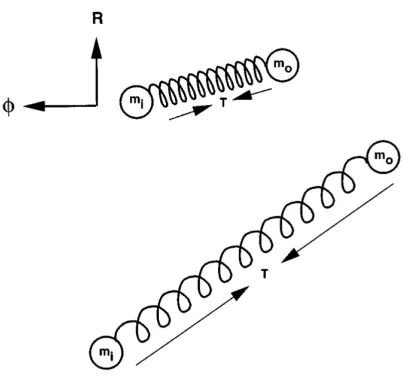
Figure 5. Two masses in orbit connected by a weak spring. The spring exerts tension forceT resulting in a transfer of angular momentum from the inner massmi to the outer massmo. If the spring is weak, the transfer
results in an instability asmi loses angular momentum, drops through more rapidly rotating inner orbits, and
moves further ahead. The outer massmogains angular momentum, moves through slower outer orbits, and drops
further behind. The spring tension increases and the process runs away (figure and caption from Balbus & Hawley 1998).
5.3 MRI
In the presence of magnetic fields, the field lines act like springs connecting different annuli within the disk. Fig. 5 illustrates the basic principle. If a weak pull exists between two masses in adjacent annuli of the disk,miandmo, the inner mass element will loose angular momentum and hence drift even
further inward, while the outer mass element gains angular momentum and drifts further outward. The new orbital velocity of the inner mass element is even higher than before (presuming thatΩdecreases withr), while the new orbital velocity of the outer element is even smaller. This effect thus enhances the velocity difference between the two masses in adjacent annuli, giving rise to an instability. The instability is generally referred to as magneto-rotational instability and has been described first by Balbus & Hawley (Balbus & Hawley (1998) - hence we often refer to it as Balbus-Hawley instability). A prerequisite for a magnetised disk to be linearly unstable is that the orbital velocity decreases with radius
d
dr(Ω)<0 , (48)
a condition clearly satisfied in Keplerian disks. In addition, the disk needs to be ionised to a certain degree since neutral gas does not couple efficiently to the magnetic field lines. The critical ionisation degree isne/ntot∼10−12to sustain turbulence generation by the magneto-rotational instability (Sano & Stone 2002).
numerical effects becomes then a challenge. However, from simulations it seems that α could be consistent with a value of∼10−2as inferred from observations.
AcknowledgementsThe author is indepted to Kees Dullemond who once explained the basic physics of viscous accretion disks to him in just half an hour. The research leading to these results has received funding from the European Union Seventh Framework Programme FP7-2011 under grant agreement no 284405.
References
Balbus, S. A. & Hawley, J. F. 1998, Reviews of Modern Physics, 70, 1
Beckwith, S., Sargent, A. I., Scoville, N. Z., et al. 1986, ApJ, 309, 755
Koerner, D. W., Sargent, A. I., & Beckwith, S. V. W. 1993, Icarus, 106, 2
Mannings, V., Koerner, D. W., & Sargent, A. I. 1997, Nature, 388, 555
O’Dell, C. R., Wen, Z., Hu, X., & Hester, J. J. 1992, in Bulletin of the American Astronomical Society, Vol. 24, American Astronomical Society Meeting Abstracts, 1147
Rodriguez, L. F., Canto, J., Torrelles, J. M., Gomez, J. F., & Ho, P. T. P. 1992, ApJL, 393, L29
Sano, T. & Stone, J. M. 2002, ApJ, 570, 314
Sargent, A. I. & Beckwith, S. 1987, ApJ, 323, 294
Shakura, N. I. & Sunyaev, R. A. 1973, A&A, 24, 337
Shu, F. H. 1977, ApJ, 214, 488