INTERFEROMETRIC ISAR IMAGING ON SQUINT MODEL
C. Z. Ma†,T. S. Yeo, and H. S. Tan
Department of Electrical and Computer Engineering National University of Singapore
Singapore
G. Y. Lu
Telecommunication Engineering Department Xi’an Institute of Post and Telecommunications China
Abstract—Conventional interferometric inverse synthetic aperture radar three dimensional imaging only consider broadside imaging condition. In this paper, squint model imaging configuration is discussed and the coordinate transform equation is given. The ISAR range profile envelope alignment problem among different antennas are also discussed. Simulation results show the effectiveness of our proposed method.
1. INTRODUCTION
Inverse Synthetic Aperture Radar (ISAR) imaging has received much attention in the past three decades [1–6]. Its high range resolution is attained by transmitting a wideband signal while it’s cross range resolution is dependent on the relative rotation between the radar and the target. It is difficult to obtain a good quality ISAR image if the targets are cooperating and/or maneuvering [3–6]. For non-cooperative targets, the targets’ rotation angle cannot be obtained and therefore, the cross range scale is not known. And for maneuvering targets, the rotational axis and the rotational speed of the target relative to the radar is time varying, which means that the Doppler
126 Ma et al.
is time varying, and therefore, time frequency analysis must be used to coherently integrate the signals to form a fine ISAR image. On the other hand, the range-Doppler plane may not coincide with the target’s conventional range and cross-range plane, and this induces difficulty for target identification.
To overcome the above drawbacks, 3-D interferometric ISAR imaging known as InISAR are proposed [7–12].
Generally three antennas are used and the target is assumed to be located at the broadside of the antennas. The phase difference of a scatterer between two different antennas can be used to determine its cross range position. For slant range target, it is assumed that the antennas rotate mechanically to steer the antenna beam towards the target and maintain the broadside assumption. Sometimes, it may not be practical or convenient to rotate the antenna. In this paper, we discuss the three dimensional imaging of a slant range target.
2. SIGNAL MODEL
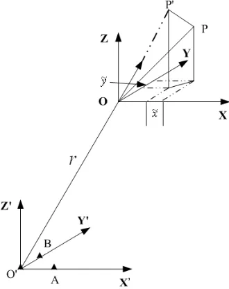
In this paper, a vector is denoted by a small bold letter or a letter with an overhead arrow, while scatterer’s position and the coordinate system are denoted by capital letters. The geometry of the three dimensional ISAR imaging based on three antennas is shown in Fig. 1. The origin of the three dimensional coordinate system (X, Y, Z) is denoted asO. The transmitting antenna also acts as a receiving antenna is located at the origin. The other two receiving antennas A, B are located in the
X and Y axis and denoted as antenna 1 and antenna 2 respectively, and the distance from bothA andB toO isd.
A local coordinate system (X, Y, Z) on the target parallel to the radar coordinate system is taken as reference, where the local origin is denoted as O. PointP located in (x, y, z) is expressed as p=−−→OP.
Let the transmitted signal from the antenna O be ˜s(t) = exp(j2πf t). The back scattered signals from scatterer P received at antennas O and A are
sp0(t) = exp
j2πf
t−2rp0 c
, (1)
and
sp1(t) = exp
j2πf
t−rp0+rp1 c
, (2)
respectively, whererp0 =|
−−→
OP|=|−−→OO+−−→OP|=|r+p|,rp1 =|−→AP|=
Figure 1. Geometry of the radar and the target.
frequency. Let the signal from the receive antenna 0 be the reference signal, then we have
s∗p0(t)sp1(t) = exp
j2πfrp0−rp1 c
. (3)
The difference betweenrp0 and rp1 is
∆r=rp0−rp1 = |r+p| − |r+p−d|
= (r+p)
T(r+p)−(r+p−d)T(r+p−d)
rp0+rp1
= 2(r+p)
Td−dTd
rp0+rp1
. (4)
For simplicity, the received signals of the two antennas are expressed in an array representation as
sp =sp0(t)×
1, ej2π
2(r+p)Td−dTd
λ(rp0+rp1)
T
. (5)
128 Ma et al.
is
sq =e−j4π
rq0(t)
λ ×
1, ej2π
2rTd−dTd
λ(rq0+rq1)
T
. (6)
LetQbe the focussing point and after compensation using sq,sp
becomes
ˆ
sp(t) = s∗q(t)sp(t)
= e−j4πrp
0(t)−rq0(t)
λ ×
1, ej2π
2(r+p)Td−dTd
λ(rp0+rp1) −
2rTd−dTd
λ(rq0+rq1)
T
, (7)
whereexpress element wise product. Now let’s consider simplifying the phase in the above array signal.
∆rQP =
2(r+p)Td−dTd (rp0+rp1) −
2rTd−dTd (rq0+rq1)
=
2(r+p)Td−dTd(r
q0+rq1)−(2rTd−dTd)(rp0+rp1)
(rp0+rp1)(rq0+rq1)
≈ 2rTd(rq0+rq1−rp0−rp1) + 2pTd(rq0+rq1)
+dTd(rp0+rp1−rq0−rq1)
/(4˜r2), (8)
where ˜r ≈rp0.
We also have
2rTd(rq0+rq1−rp0−rp1)
4˜r2 ≈ −n
T
0dpTn0/r,˜ (9)
2pTd(rq0+rq1)
4˜r2 =
pTd ˜
r , (10)
and
dTd(rp0+rp1−rq0−rq1)
4˜r2 =
dTdpTn0
2˜r2 , (11)
here we use the approximation r/r˜ ≈ n0, rq0 −rp0 ≈ −pTn0 and rq1−rp1 ≈ −pTn0. Therefore,
∆rQP = −
nT0dpTn0+pTd
˜
r +
dTdpTn0
2˜r2
(p−pTn0n0)Td
˜
r (12)
can be simplified to
ˆ
sp(t) =e−j4π
rp0(t)−rq0(t)
λ ×
1, ej2π(p−p
Tn
0n0)Td
λr˜ (13)
It should be noted that the above equation (13) holds only when (1) the target is located in far field and the size of the target is small, (2) the motion of the target in the range direction is small.
3. THREE DIMENSIONAL IMAGING ALGORITHMS The position of scatterer P relative to Q along X direction can be obtained by comparing the phase of antenna 1 and antenna 0’s received signals. Similarly, the position ofP relative toQalong theY direction can also be obtained. Together with the range information obtained by wide band pulse compression, the three dimensional position of scatterer P relative to Q can be obtained. The phase of the signal of P can be obtained by first carrying out ISAR imaging of the three antennas’ signals. What we need to pay more attention on is to retain the phase information during the ISAR imaging process as this can be used to deduce the scatterer’s position.
In ISAR imaging, the first step is envelope alignment. Because the delays rp0 et al. are time varying, the echo’s envelopes are shifted
withtime. Cross range signal processing can only be done after the signals’ envelopes are aligned. For a three-antenna case, compared to one antenna ISAR imaging, what we need to know is that at any time instance, whether the different antenna’s one dimensional range profiles are aligned or not. For slant range imaging condition, it is obvious that envelope alignment is needed as the distances of the target to the three antennas are different, and as the difference in distance is comparable to range resolution, therefore range alignment is needed for the signals from the different antennas.
According to (13), the phase differenceϕx between antenna 0 and
antenna 1 is
ϕx =
2π(p−pTn0n0)Td
λr˜ , (14)
and this can be obtained by ISAR imaging. Similarly, the phase differenceϕy between antenna 0 and antenna 2 can also be obtained.
Denote−−→PP =p−pTn
0n0={x,˜ y,˜ z˜}, r=pTn0,n0={nx, ny, nz},
and p={x, y, z}, then we have ˜
x = ϕx
λr˜
130 Ma et al.
˜
y = ϕy
λr˜
2πd, (16)
˜
x = x−rnx, (17)
˜
y = y−rny, (18)
UsingpTn
0 =r, it is easy to obtain
x = ˜x+rnx, (19)
y = ˜y+rny, (20)
z = r−xnx−yny
nz
. (21)
As the period of phase is of modulo 2π, in order to ensure that there exists an unique relationship between ˜xandϕ, one should ensure that 2πxd˜
λ˜r
< π. Therefore, the maximum cross range non-ambiguous widthis
˜
x∈X=
−λ˜r 2d,
λ˜r
2d . (22)
In the above discussion, we have also assumed that the radar line of sight vectorn0 is obtained by other system.
30 20 10 0 10 20 30
30 20 10 0 10 20 30
X axis, Meter
Y
axis, Meter
Figure 2. Original target’s image on theXY plane.
30 20 10 0 10 20 30
30 20 10 0 10 20 30
X axis, Meter
Z
axis, Meter
Figure 3. Original target’s image on theXZ plane.
4. SIMULATION RESULTS
20 15 10 5 0 5 10 15 20 20
15 10 5 0 5 10 15 20
Y axis, Meter
Z
axis, Meter
Figure 4. Original target’s image on theY Z plane.
Figure 5. Original target’s three dimensional image.
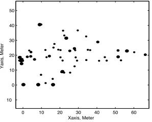
cross unambiguous distance is 105.8 m. The target is composed of 69 scatterers and is placed in the [1, 1, 1] direction. Fig. 2, Fig. 3, Fig. 4 and Fig. 5 depict the three projected images and three dimensional image of the original target. The target moves with a velocity of [3,32,−32] m per second. The data collection time is 5 s, therefore the angle of rotation is 0.6492◦ which results in a nominal cross range resolution of about 0.3536 m. An isolated scatterer is used to do motion compensation and the ISAR image of antenna 0 is shown in Fig. 6. The reconstructed three projected images and three dimensional image are shown in Fig. 7, Fig. 8, Fig. 9 and Fig. 10. It can be seen that the reconstructed three dimensional image is similar to that of the original target’s image.
Figure 6. Target’s ISAR image.
0 10 20 30 40 50 60
10 0 10 20 30 40 50
Xaxis, Meter
Yaxis, Meter
132 Ma et al.
0 10 20 30 40 50 60 10
0 10 20 30 40 50
Xaxis, Meter
Zaxis, Meter
Figure 8. Reconstructed tar-get’s image on theXZ plane.
0 5 10 15 20 25 30 35 40 0
5 10 15 20 25 30 35 40
Yaxis, Meter
Zaxis, Meter
Figure 9. Reconstructed tar-get’s image on the Y Z plane.
Figure 10. Reconstructed target’s three dimensional image.
5. CONCLUSIONS
In this paper, we have derived a three dimensional imaging formula for slant range targets. Generally, envelope alignment between different antennas is needed. Simulation results show the effectiveness of our proposed method.
ACKNOWLEDGMENT
REFERENCES
1. Chen, C. C. and H. C. Andrews, “Target-motion-induced radar imaging,” IEEE Trans. Aerosp. Electron. Syst., Vol. 16, 2–14, Jan. 1980.
2. Walker, J. L., “Range-Doppler imaging of rotating objects,”IEEE Trans. Aerosp. Electron. Syst., Vol. 16, 23–52, Jan. 1980.
3. Bao, Z., G. Y. Wang, and L. Luo, “Inverse synthetic aperture radar imaging of maneuvering targets,”Opt. Eng., Vol. 37, 1582, 1998.
4. Wang, G. Y. and Z. Bao, “ISAR imaging of maneuvering targets based on chirplet decomposition,”Opt. Eng., Vol. 38, 1534–1541, 1999.
5. Wang, Y., H. Lin, and V. C. Chen, “ISAR motion compensation via adaptive joint time-frequency techniques,” IEEE Trans. Aerospace and Elec. Sys., Vol. 34, No. 2, 670–677, 1998.
6. Chen, V. C. and S. Qian, “Joint time-frequency transform for radar range doppler imaging,” IEEE Trans. Aerospace and Elec. Sys., Vol. 34, No. 2, 486–499, Feb. 1998.
7. Ma, C. Z., “Researchon radar three dimensional imaging techniques,” Ph.D. thesis, Xidian University, 1999.
8. Wang, G. Y., X. G. Xia, and V. C. Chen, “Three dimensional ISAR imaging of maneuvering targets using three receivers,”IEEE Trans. Image Processing, Vol. 10, 436–447, Mar. 2001.
9. Xu, X. J. and R. M. Narayanan, “Three-dimensional interferomet-ric ISAR imaging for target scattering diagnosis and modeling,” IEEE Trans. Image Processing, Vol. 10, 1094–1102, July 2001. 10. Zhang, Q., C. Z. Ma, T. Zhang, and S. H. Zhang, “Research on
radar three dimensional imaging techniques based on interferomet-ric techniques,” Journal of Electronic and Information, Vol. 23, 890–898, Sept. 2001.
11. Zhang, Q., T. S. Yeo, G. Du, and S. H. Zhang, “Estimation of three-dimensional motion parameters in interferometric ISAR imaging,”IEEE Trans. Geosci. Remote Sensing, Vol. 42, 292–300, Feb. 2004.