R e v i e w
Open Access
Optimal resource allocation in wireless
communication and networking
Alejandro Ribeiro
Abstract
Optimal design of wireless systems in the presence of fading involves the instantaneous allocation of resources such as power and frequency with the ultimate goal of maximizing long term system properties such as ergodic capacities and average power consumptions. This yields a distinctive problem structure where long term average variables are determined by the expectation of a not necessarily concave functional of the resource allocation functions. Despite their lack of concavity it can be proven that these problems have null duality gap under mild conditions permitting their solution in the dual domain. This affords a significant reduction in complexity due to the simpler structure of the dual function. The article discusses the problem simplifications that arise by working in the dual domain and reviews algorithms that can determine optimal operating points with relatively lightweight computations. Throughout the article concepts are illustrated with the optimal design of a frequency division broadcast channel.
Introduction
Operating variables of a wireless system can be separated in two types. Resource allocation variablesp(h) determine instantaneous allocation of resources like frequencies and transmitted powers as a function of the fading coefficient h. Average variablesxcapture system’s performance over a large period of time and are related to instantaneous resource allocations via ergodic averages. A generic rep-resentation of the relationship between instantaneous and average variables is
x≤E[f1(h,p(h))] , (1)
wheref1(h,p(h))is a vector function that maps channel hand resource allocationp(h) to instantaneous perfor-mance f1(h,p(h)). The system’s design goal is to select resource allocationsp(h) to maximize ergodic variablesx in some sense.
An example of a relationship having the form in (1) is a code division multiple access channel in which caseh denotes the vector of channel coefficients,p(h) the instan-taneous transmitted power,f1(h,p(h))the instantaneous communication rate determined by the signal to interfer-ence plus noise ratio, andxthe ergodic rates determined by the expectation of the instantaneous rates. The design
Correspondence: [email protected]
Department of Electrical and Systems Engineering, University of Pennsylvania, 200 S. 33rd St., Philadelphia, PA, 19096, USA
goal is to allocate instantaneous powerp(h) subject to a power constraint so as to maximize a utility of the ergodic rate vectorx. This interplay of instantaneous actions to optimize long term performance is pervasive in wireless systems. A brief list of examples includes optimization of orthogonal frequency division multiplexing [1], beam-forming [2,3], cognitive radio [4,5], random access [6,7], communication with imperfect channel state informa-tion (CSI) [8,9], and various flavors of wireless network optimization [10-18].
In many cases of interest the functionsf1(h,p(h))are nonconcave and as a consequence finding the resource allocation distribution p∗(h) that maximizes x requires solution of a nonconvex optimization problem. This is fur-ther complicated by the fact that since fading channelsh take on a continuum of values there is an infinite num-ber ofp∗(h)variables to be determined. A simple escape to this problem is to allow for time sharing in order to make the range ofE[f1(h,p(h))] convex and permit solu-tion in the dual domain without loss of optimality. While the nonconcave functionf1(h,p(h))still complicates mat-ters, working in the dual domain makes solution, if not necessarily simple, at least substantially simpler. However, time sharing is not easy to implement in fading channels.
In this article, we review a general methodology that can be used to solve optimal resource alloca-tion problems in wireless communicaalloca-tions and
working without resorting to time sharing [19,20]. The fundamental observation is that the range of E[f1(h,p(h))] is convex if the probability distribution of the channel h contains no points of positive probabil-ity (Section “Dualprobabil-ity in wireless systems optimization”). This observation can be leveraged to show lack of dual-ity gap of general optimal resource allocation problems (Theorem 1) making primal and dual problems equiva-lent. The dual problem is simpler to solve and its solu-tion can be used to recover primal variables (Secsolu-tion “Recovery of optimal primal variables”) with reduced computational complexity due to the inherently sep-arable structure of the problem Lagrangians (Section “Separability”). We emphasize that this reduction in com-plexity, as in the case of time sharing, just means that the problem becomes simpler to solve. In many cases it also becomes simple to solve, but this is not necessarily the case.
We also discuss a stochastic optimization algorithm to determine optimal dual variables that can operate without knowledge of the channel probability distri-bution (Section “Dual descent algorithms”). This algo-rithm is known to almost surely converge to optimal operating points in an ergodic sense (Theorem 5). Throughout the article concepts are illustrated with the optimal design of a frequency division broadcast channel (Section “Frequency division broadcast channel” in “Optimal wireless system design”, Section “Frequency division broadcast channel” in “Recovery of optimal pri-mal variables”, and Section “Frequency division broadcast channel” in “Dual descent algorithms”).
One of the best known resource allocation problems in wireless communications concerns the distribution of power on a block fading channel using capacity-achieving codes. The solution to this problem is easy to derive and is well known to reduce to waterfill-ing across the fadwaterfill-ing gain, e.g., [21, p. 245]. Since this article can be considered as an attempt to generalize this solution methodology to general wireless commu-nication and networking problems it is instructive to close this introduction by reviewing the derivation of the waterfilling solution. This is pursued in the following section.
Power allocation in a point-to-point channel
Consider a transmitter having access to perfect CSI h
that it uses to select a transmitted powerp(h)to convey information to a receiver. Using a capacity achieving code the instantaneous channel rate for fading realizationhis
r(h) = log(1+ hp(h)/N0) where N0 denotes the noise
power at the receiver end. A common goal is to maximize the average rate r := E[r(h)] with respect to the prob-ability distributionmh(h) of the channel gain h—which
is an accurate approximation of the long term average
rate—subject to an average power constraintP0. We can
formulate this problem as the optimization program
P=maxE
log
1+ hp(h)
N0
s.t. E[p(h)]≤q0. (2)
In most cases the fading channelhtakes on a continuum of values. Therefore, solving (2) requires the determina-tion of a power allocadetermina-tion funcdetermina-tion p : R+ → R+ that maps nonnegative fading coefficients to nonnega-tive power allocations. This means that (2) is an infi-nite dimensional optimization problem which in principle could be difficult to solve. Nevertheless, the solution to this program is easy to derive and given by waterfilling as we already mentioned. The widespread knowledge of the waterfilling solution masks the fact that is is rather remarkable that (2) is easy to solve and begs the question of what are the properties that make it so. Let us then review the derivation of the waterfilling solution in order to pinpoint these properties.
To solve (2) we work in the dual domain. To work in the dual domain we need to introduce the Lagrangian, the dual function, and the dual problem. Introduce then the nonnegative dual variable λ ∈ R+ and define the Lagrangian associated with the optimization problem in (2) as
L(p,λ)=E
log
1+hp(h)
N0
+λ[q0−E[p(h)]] .
(3)
The dual function is defined as the maximum value of the Lagrangian across all functions p : R+ → R+, which upon definingP := {p : p(h) ≥ 0} as the set of nonnegative functions can be defined as
g(λ):=max
p∈P L(p,λ)
=max
p∈P E
log
1+ hp(h)
N0
+λ[q0−E[p(h)] ] .
(4)
The dual problem corresponds to the minimization of the dual function with respect to all nonnegative multipliersλ,
D=min
λ≥0g(λ)=minλ≥0maxp∈P L(p,λ). (5)
Since the objective in (2) is concave with respect to variablesp(h)and the constraint is linear inp(h)the opti-mization problem in (2) is convex and as such it has null duality gap in the sense thatP=D.
This function is defined as the one that maximizes the Lagrangian for given dual variableλ
p(λ)=argmax
p∈P L(p,λ). (6)
Using the definition of the Lagrangian maximizer function we can write the dual function asg(λ)=L(p(λ),λ).
Computing valuesp(h,λ)of the Lagrangian maximizer functionp(λ)is easy. To see that this is true rewrite the Lagrangian in (3) so that there is only one expectation
L(p,λ)=E
With the Lagrangian written in this form we can see that the maximization ofL(p,λ)required by (6) can be decomposed in maximizations for each individual channel realization,
That the equality in (8) is true is a consequence of the fact that the expectation operator is linear and that there are no constraints coupling the selection of valuesp(h1)and
p(h2) for different channel realizations h1 = h2.
Func-tional valuesp(h)in both sides of (8) are required to be nonnegative but other than that we can selectp(h1)and
p(h2)independently of each other as indicated in the right hand side of (8).
Since the right hand side of (8) states that to maximize the Lagrangian we can select functional valuesp(h) inde-pendently of each other, valuesp(h,λ)of the Lagrangian maximizer functionp(λ)defined in (6) are given by
p(h,λ)=argmax
The similarity between (6) and (9) is deceiving as the latter is a much easier problem to solve that involves a single variable. To find the Lagrangian maximizer value
p(h,λ)operating from (9) it suffices to solve for the null of the derivative with respect top(h). Doing this yields the Lagrangian maximizer onto nonnegative reals, which is needed because of the constraintp(h)≥0.
Of particular interest is the Lagrangian maximizer func-tionp(λ∗)corresponding to the optimal Lagrange multi-plierλ∗:= argminλ≥0g(λ). Returning to the definition of
the dual function in (4) we can boundD=g(λ∗)as
D=max
p∈PL(p,λ
∗)≥Lp∗,λ∗. (11)
Indeed, sinceDis given by a Lagrangian maximization it must equal or exceed the values of the Lagrangian for any functionp, and for the optimal functionp∗in particular. Considering the explicit Lagrangian expression in (3) we can writeL(p∗,λ∗)as
Observe that since p∗ is the optimal power allocation function it must satisfy the power constraint implying that it must be q0 −E[p∗(h)] ≥ 0. Since the optimal dual
variable satisfiesλ∗≥0 their product is also nonnegative allowing us to transform (12) into the bound
Lp∗,λ∗≥E
where the equality is true becausePandp∗are the otpimal value and arguments of the primal optimization problem (2). Combining the bounds in (11) and (13) yields
D=max
p∈PL
p,λ∗≥Lp∗,λ∗≥P. (14)
Using the equivalenceP=Dof primal and dual optimum values it follows that the inequalities in (13) must hold as equalities. The equality maxp∈PL(p,λ∗) = L(p∗,λ∗), in
particular, implies that the functionp∗ is the Lagrangian maximizing function corresponding toλ=λ∗, i.e.,
p∗=pλ∗=argmax
p L
p,λ∗. (15)
The important consequence of (15) follows from the fact that the Lagrangian maximizer functionp(λ∗)is easy to compute using the decomposition in (9). By extension, if the optimal multiplierλ∗is available, computation of the optimal power allocation functionp∗also becomes easy. Indeed, making λ = λ∗in (9) we can determine values
Recapping the derivation of the optimal power alloca-tionp∗, we see that there are three conditions that make (18) simple:
(C1) Since the optimization problem is convex it is equivalent to its Lagrangian dual implying that optimal primal variables can be determined as Lagrangian maximizers associated with the optimal multiplierλ∗[cf. (11)–(15)].
(C2) Due to the separable structure of the Lagrangian, determination of the optimal power allocation function is carried out through the solution of per-fading state subproblems [cf. (6)–(9)]. (C3) Because there is a finite number of constraints the
dual function is finite dimensional even though there is an infinite number of primal variables.
Most optimization problems in wireless systems are separable in the sense of (C2) and have a finite number of constraints as [cf. (C3)] but are typically not convex [cf. (C1)].
To illustrate this latter point consider a simple variation of (2) where instead of using capacity achieving codes we use adaptive modulation and coding (AMC) relying on a set ofLcommunication modes. Thel-th mode supports a rateαland is used when the signal to noise ratio (SNR)
at the receiver end is betweenβl−1 andβl. Lettingγ be
the received SNR andI(E)denote the indicator function of the eventE, the communication rate functionC(γ )for AMC can be written as
CAMC(γ )=
L
l=1 αlI
βl ≤γ < βl+1
. (17)
The corresponding optimal power allocation problem subject to average power constraintq0can now be
formu-lated as
P=maxE
L
l=1 αlI
βl≤
hp(h) N0 < βl+1
s.t. E[p(h)]≤q0. (18)
Similar to (2) the dual function of the optimization prob-lem in (18) is one dimensional and its Lagrangian is sepa-rable in the sense that we can find Lagrangian maximizers by performing per-fading state maximizations. Alas, the problem is not convex because the AMC rate function
C(γ )is not concave, in fact, it is not even continuous. Since it does not satisfy (C1), solving (18) in the dual domain is not possible in principle. Nevertheless the condition that allows determination of p∗(h) as the Lagrangian maximizerp(h,λ∗)[cf. (16)] is not the convex-ity of the primal problem but the lack of dualconvex-ity gap. We’ll see in Section “Duality in wireless systems optimization” that this problem does have null duality gap as long as
the probability distribution of the channel h contains no points of strictly positive probability. Thus, the solu-tion methodology in (3)-(16) can be applied to solve (18) despite the discontinuous AMC rate functionC(γ ). This is actually a quite generic property that holds true for opti-mization problems where nonconcave functions appear inside expectations. We introduce this generic problem formulation in the next section.
Optimal wireless system design
Let us return to the relationship in (1) where hdenotes the random fading state that ranges on a continuous space H,p(h) the instantaneous resource allocation,f1(h,p(h)) a vector function mapping hand p(h) to instantaneous system performance, andxan ergodic average. The expec-tation in (1) is with respect to the joint probability distri-butionmh(h)of the vector channelh.
It is convenient to think off1(h,p(h))as a family of func-tions indexed by the parameterhwithp(h) denoting the corresponding variables. Notice that there is one vector p(h) per fading state h, which translates into an infinite number of resource allocation variables ifhtakes on an infinite number of values. Consequently, it is adequate to refer to the set p := {p(h)}h∈H of all resource alloca-tions as the resource allocation function. The number of ergodic limitsxof interest, on the other hand, is assumed finite.
Instantaneous resource allocationsp(h) are further con-strained to a given bounded setP(h). These restrictions define a set of admissible resource allocation functions that we denote as
P:= {p:p(h)∈P(h), for allh∈H}. (19)
Variablesp(h) determine system performance over short periods of times. As such, they are of interest to the sys-tem designer but transparent to the end user except to the extent that they determine the value of ergodic vari-ablesx. Therefore, we adopt as our design objective the maximization of a concave utility function f0(x) of the ergodic averagex. Putting these preliminaries together we write the following program as an abstract formulation of optimal resource allocation problems in wireless systems
P=max f0(x)
s.t. x≤E[f1(h,p(h))] , f2(x)≥0,
x∈X, p∈P, (20)
not necessarily convex. The sets X andP are assumed compact to guarantee thatxandp(h) are finite. For the expectation in (20) to exist we need to havef1(h,p(h)) integrable with respect to the probability distribution
mh(h) of the vector channel h. This imposes a (mild) restriction on the functionsf1(h,p(h))and the power allo-cation functionp. Integrability is weaker than continuity.
For future reference definex∗andp∗as the arguments that solve (20)
(x∗,p∗)=argmax f0(x)
s.t x≤E[f1(h,p(h))] , f2(x)≥0, x∈X, p∈P. (21)
The configuration pair (x∗,p∗) attains the optimum value P = f0(x∗) and satisfies the constraints x∗ ≤ E[f1(h,p∗(h))] and f2(x∗) ≥ 0 as well as the set con-straintsx∗∈X, andp∗∈P. Observe that the pair(x∗,p∗) need not be unique. It may be, and it is actually a common occurrence in practice, that more than one configuration is optimal. Thus, (21) does not define a pair of variables but a set of pairs of optimal configurations. As it does not lead to confusion we use(x∗,p∗)to represent both, the set of optimal configurations and an arbitrary element of this set.
To write the Lagrangian we introduce a nonnegative Lagrange multiplier=λT1,λT2 Twhereλ1≥0is
asso-ciated with the constraintx≤E[f1(h,p(h))] andλ2≥0
with the constraintf2(x). The Lagrangian of the primal optimization problem in (20) is then defined as
L(x,p,):=f0(x)+λT1[E(f1(h,p(h)))−x]+λT2f2(x).
(22)
The corresponding dual function is the maximum of the Lagrangian with respect to primal variablesx ∈ X and p∈P
g():= max
x∈X,p∈PL(x,p,). (23)
The dual problem is defined as the minimum value of the dual function over all nonnegative dual variables
D=min
≥0 g(), (24)
and the optimal dual variables are defined as the argu-ments that achieve the minimum in (24)
∗:=argmin
≥0 g(). (25)
Notice that the optimal dual argument∗is a set as in the case of the primal optimal arguments because there may be more than one vector that achieves the minimum in (24). As we do with the optimal primal variables(x∗,p∗), we use∗to denote the set of optimal dual variables and an arbitrary element of this set. A particular example of this generic problem formulation is presented next.
Frequency division broadcast channel
A common access point (AP) administers a power budget
q0to communicate with a group ofJnodes. The physical
layer uses frequency division so that at most one termi-nal can be active at any given point in time. The goal is to design an algorithm that allocates power and fre-quency to maximize a given ergodic rate utility metric while ensuring that rates are at leastrmin and not more
thanrmax.
Denote ashi the channel to terminal iand define the
vector h := h1. . .,hJ T grouping all channel
realiza-tions. In any time slot the AP observes the realization hof the fading channel and decides on suitable power allocations pi(h) and frequency assignments αi(h).
Fre-quency assignmentsαi(h)are indicator variablesαi(h) ∈ {0, 1} that take value αi(h) = 1 when information is
transmitted to node i and αi(h) = 0 otherwise. If αi(h) = 1 communication towards i ensues at power
pi(h) resulting in a communication rate C(hipi(h)/N0)
determined by the SNRhipi(h)/N0. The specific form of
the functionC(hipi(h)/N0)mapping channels and powers
to transmission rates depends on the type of modula-tion and codes used. One possibility is to select capacity achieving codes leading to C(hipi(h)/N0) = log(1 +
hipi(h)/N0). A more practical choice is to use AMC in
which case C(hipi(h)/N0) = CAMC(hipi(h)/N0) with
CAMC(hipi(h)/N0)as given in (17).
Regardless of the specific form ofC(hipi(h)/N0)we can
write the ergodic rate of terminalias
ri=E
αi(h)C
hipi(h)
N0
. (26)
The factor C(hipi(h)/N0) is the instantaneous rate
achieved if information is conveyed. The factor αi(h)
indicates wether this information is indeed conveyed or not. The expectation weights the instantaneous capacity across fading states and is equivalent to the consideration of an infinite horizon time average.
Similarly,pi(h)denotes the power allocated for
commu-nication with nodei, but this communication is attempted only if αi(h) = 1. Thus, the instantaneous power
uti-lized to communicate withifor channel realizationhis
αi(h)pi(h). The total instantaneous power is the sum of
these products for alliand the long term average power consumption can be approximated as the expectation
E J
i=1
αi(h)pi(h)
≤q0, (27)
that according to the problem statement cannot exceed the budgetq0.
To avoid collisions between communication attempts the indicator variables αi(h) are restricted so that at
α1(h),. . .,αJ(h) T corresponding to values of the
function α:=α1,. . .,αJ T and introduce the set of
vector functions
A:=α:α(h)∈ {0, 1}, 1Tα(h)≤1. (28)
We can now express the frequency exclusion constraints asα∈A.
We still need to model the restriction that the achieved capacityrineeds to be betweenrminandrmaxbut this is
easily modeled as the constraintrmin≤ri ≤rmax.
Defin-We finally introduce a monotonic nondecreasing utility functionU(ri)to measure the value of rateriand formally
state our design goal as the maximization of the aggregate utilityJi=1U(ri). Using the definitions in (26)–(29) the
operating point that maximizes this aggregate utility for a frequency division broadcast channel follows from the solution of the optimization problem
P=max
where we relaxed the rate expression in (26) to an inequal-ity constraint, which we can do without loss of optimalinequal-ity because the utilityU(ri)is monotonic nondecreasing.
The problem formulation in (30) is of the form in (20). The ergodic ratesrin (30) are represented by the ergodic variables x in (20) whereas the power and frequency allocation functions p andα of (30) correspond to the resource allocation function p of (20). The set Rmaps to the set X and the set A to the setP. There are no functions in (30) taking the place of the function f2(x) of (20). The functionf1(h,p(h))in (20) is a placeholder for the stacking of the functions αi(h)C(hipi(h)/N0)for
different i and the negative of the power consumptions
−J
i=1αi(h)pi(h) in (30). The power constraint q0 ≥
EJ
i=1αi(h)pi(h)
is not exactly of the form in (1) because q0 is a constant not a variable but this doesn’t
alter the fundamentals of the problem. The functions
αi(h)C(hipi(h)/N0)are not concave and the setAis not
convex. This makes the program in (30) nonconvex but is consistent with the restrictions imposed in (20).
To write the Lagrangian corresponding to this optimiza-tion problem introduce multipliers λ := λ1,. . .,λJ T
associated with the capacity constraints and μ associ-ated with the power constraint. The Lagrangian is then given by
The dual function, dual problem, and optimal dual arguments are defined as in (22)–(25) by replacing L(r,p,α,λ,μ) forL(x,p,). Since (30) is a nonconvex program we do not know if the dual problem is equiva-lent to the primal problem. We explore this issue in the following section.
Duality in wireless systems optimization
For any optimization problem the dual minimumD pro-vides an upper bound for the primal optimum value P. This is easy to see by combining the definitions of the dual function in (23) and the Lagrangian in (22) to write
g()= max
x∈X,p∈Pf0(x)+λ T
1[E(f1(h,p(h)))−x]+λT2f2(x).
(32)
Because the dual function valueg()is obtained by max-imizing the right hand side of (32), evaluating this expres-sion for arbitrary primal variables yields an upper bound ong(). Using a pair(x∗,p∗)of optimal primal arguments as this arbitrary selection yields the inequality
g()≥f0(x∗)+λT1Ef1
h,p∗(h)−x∗ +λT2f2(x∗). (33)
Since the pairx∗,p∗is optimal, it is feasible, which means that we must haveE[f1(h,p∗(h))]−x∗≥0andf2(x∗)≥ 0. Lagrange multipliers are also nonnegative according to definition. Therefore, the last two summands in the right hand side of (33) are nonnegative from which it follows that
g()≥f0(x∗)=P. (34)
The inequality in (34) is true for anyand therefore true for = ∗ in particular. It then follows that the dual optimumDupper bounds the primal optimumP,
D≥P, (35)
as we had claimed. The differenceD-Pis called the duality gap and provides an indication of the loss of optimality incurred by working in the dual domain.
For the problem in (20) the duality gap is null as long as the channel probability distributionmh(h) contains no
theorem which is a simple generalization of a similar result in [20].
Theorem 1. Let P denote the optimum value of the primal
problem(20) and D that of its dual in(24) and assume
there exists a strictly feasible point (x0,p0) that satisfies
the constraints in(20)with strict inequality. If the channel
probability distribution mh(h)contains no point of positive
probability the duality gap is null, i.e.,
P=D. (36)
The condition on the channel distribution not hav-ing points of positive probability is a mild requirement satisfied by practical fading channel models including Rayleigh, Rice, and Nakagami. The existence of a strictly feasible point(x0,p0)is a standard constraint qualification
requirement which is also not stringent in practice. In order to prove Theorem 1 we take a detour in Section “Lyapunov’s convexity theorem” to define atomic and nonatomic measures along with the pre-sentation of Lyapunov’s Convexity Theorem. The proof itself is presented in Section “Proof of Theorem 1”. The implications of Theorem 1 are discussed in Sections “Recovery of optimal primal variables” and “Dual descent algorithms”.
Lyapunov’s convexity theorem
The proof of Theorem 1 uses a theorem by Lyapunov concerning the range of nonatomic measures [22]. Mea-sures assign strictly positive values to sets of a Borel field. When all points have zero measure the measure is called nonatomic as we formally define next.
Definition 1(Nonatomic measure). Let w be a measure
defined on the Borel fieldBof subsets of a spaceX.
Mea-sure w is nonatomic if for any measurable set E0∈Bwith
w(E0) > 0, there exist a subset E of E0; i.e., E ⊂ E0, such
that w(E0) >w(E) >0.
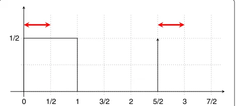
Familiar measures are probability related, e.g., the prob-ability of a set for a given channel distribution. To build intuition on the notion of nonatomic measure consider a random variableXtaking values in [ 0, 1] and [ 2, 3]. The probability of landing in each of these intervals is 1/2 andX is uniformly distributed inside each of them; see Figure 1. The spaceX is the real line, and the Borel field Bcomprises all subsets of real numbers. For every subset
E ∈ Bdefine the measure ofEas twice the integral ofx, weighted by the probability distribution ofXon the setE, i.e.,
wX(E):=2
E
xdX. (37)
Note that, except for the factor 2, the value ofwX(E)
represents the contribution of the setE to the expected value ofXand that whenEis the whole spaceX, it holds
0 1/2 1 3/2 2 5/2 3 7/2
1/2
Figure 1Nonatomic measure.The random variableXis uniformly distributed in [ 0, 1]∪[ 2, 3]. The measurewX(E):=2
ExdXis
nonatomic because all sets of nonzero probability include a smaller set of nonzero probability. Lyapunov’s convexity theorem (Theorem 2) states that the measure rangeW:= {wX(E):E∈B}is
convex. The range ofwXis the, indeed convex, interval [ 0, 3].
wX(X) = 2EX(x). According to Definition 1, wX(E) is
a nonatomic measure of elements ofB. Every subsetE0
withwX(E0) > 0 includes at least an interval(a,b). The
measure of the set E := E0−((a+b)/2,b)formed by
removing the upper half of (a,b) from E0 is wX(E) =
wX(E0)−(b−a)/2. The measure ofEsatisfieswX(E) >0
as required forwX(E)to be nonatomic.
To contrast this with an example of an atomic mea-sure consider a random variableY landing equiprobably in [ 0, 1] or 5/2; see Figure 2. In this case, the measure
wY(E) := 2
EydY is atomic because the setE0 = {5/2}
has positive measurewY(E) = 1. The only setE ⊂ E0is
the empty set whose measure is null.
The difference between the distributions ofXandY is thatYcontains a point of strictly positive probability, i.e., an atom. This implies presence of delta functions in the probability density function ofY. Or, in a rather cleaner statement the cumulative distribution function (cdf ) ofX
is continuous whereas the cdf ofYis not.
Lyapunov’s convexity theorem introduced next refers to the range of values taken by (vector) nonatomic measures.
0 1/2 1 3/2 2 5/2 3 7/2
1/2
Figure 2Atomic measure.The random variableYlands with equal probability inY=5/2 and uniformly in the interval [ 0, 1]. The measurewY(E):=2EydYis atomic because the set{1}has strictly
positive probability and no set other than the empty set is strictly included in{1}. Theorem 2 does not apply. The range ofwY(E)is the
Theorem 2(Lyapunov’s convexity theorem [22]).
Con-sider nonatomic measures w1,. . .,wnon the Borel fieldBof
subsets of a spaceXand define the vector measurew(E):=
[w1(E),. . .,wn(E)]T. The range W := {w(E):E∈B} of
the measurewis convex. I.e., ifw(E1)= w1andw(E2) =
w2, then for anyα ∈[ 0, 1]there exists E0 ∈ Bsuch that
w(E0)=αw1+(1−α)w2.
Returning to the probability measures defined in terms of the probability distributions of the random variablesX
andY, Theorem 2 asserts that the range ofwX(E), i.e., the
set of all possible values taken bywXis convex. In fact, it
is not difficult to verify that the range ofwX is the convex
interval [ 0, 3] as shown in Figure 1. Theorem 2 does not claim anything aboutwY. In this case, it is easy to see that
the range ofwY is the (non-convex) union of the intervals
[ 0, 1/2] and [ 5/2, 3]; see Figure 2.
Proof of Theorem 1
To establish zero duality gap we will consider a perturbed version of (20) obtained by perturbing the constraints used to define the Lagrangian in (22). The perturbation function P() assigns to each (perturbation) parame-ter set := δT1,δT2 T the solution of the (perturbed) optimization problem
P()=max f0(x)
s.t. E[f1(h,p(h))]−x≥δ1, f2(x)≥δ2, x∈X, p∈P. (38)
The perturbed problem in (38) can be interpreted as a modified version of (20), where we allow the constraints to be violated byamounts. To prove that the duality gap is zero, it suffices to show thatP()is a concave function of; see, e.g., [23].
Let =[δT1,δT2]T and =[δ1T,δ2T]T be an arbi-trary given pair of perturbations. Let (x,p) be a pair of ergodic limits and resource allocation variables achieving the optimum value P() corresponding to perturbation
. Likewise, denote as(x,p)a pair that achieves the opti-mum valueP()corresponding to perturbation. For arbitraryα∈[ 0, 1], we are interested in the solution of (38) under perturbationα :=α+(1−α). In particular, to show that the perturbation functionP()is concave we need to establish that
P(α)=Pα+(1−α)
≥αP()+(1−α)P. (39)
The roadblock to establish concavity of the perturbation functions is the constraint x ≤ E[f1(h,p(h))]. More
specifically, the difficulty with this constraint is the ergodic limitE[f1(h,p(h))]. Let us then isolate the challenge by
defining the ergodic limit span
Y:=y ∃p∈Pfor whichy=E[f1(h,p(h))]. (40)
The setYcontains all the possible values that the expec-tationE[f1(h,p(h))] can take as the resource allocation
function p varies over the admissible set P. When the channel distributionmh(h)contains no points of positive probability, the setYis convex as we claim in the following theorem.
Theorem 3. LetYbe ergodic limit span set in(40). If the
channel probability distribution mh(h)contains no point
of positive probability the setYis convex.
Before proving Theorem 3 let us apply it to complete the proof of Theorem 1. For doing that consider two arbitrary pointsy∈Yandy∈Y. If these points belong toYthere exist respective resource allocation functionsp ∈ P and p∈Psuch that
y=E[f1(h,p(h))] , y=Ef1(h,p(h)) . (41)
IfYis a convex set as claimed by Theorem 3, we must have that for any givenαthe pointyα := αy+(1−α)yalso belongs toY. In turn, this means there exists a resource allocation functionpα∈Pfor which
yα:=αE[f1(h,p(h))]+(1−α)Ef1h,p(h)
=E[f1(h,pα(h))] . (42)
Further define the ergodic limit convex combinationxα:=
αx+(1− α)x. We first show that the pair (xα,pα) is feasible for the problem for perturbationα.
The convex combination satisfies the constraintxα ∈X because the setX is convex. We also havef2(xα) ≥ δ2,α
because the function f2(x) is concave. To see that this is true simply notice that concavity of f2(x)implies that f2(xα) = f2[αx+(1− α)x]≥ αf2(x)+(1 −α)f2(x). Butf2(x) ≥ δ2andf2(x) ≥ δ2becausexandxare fea-sible in (38) with perturbations and . Substituting these latter two inequalities into the previous one yields f2(xα)≥αδ2+(1−α)δ2=δ2,αaccording to the definition
ofα.
We are left to show that the pair (xα,pα) satisfies the constraintE[f1(h,p(h))]−x≤ δ1,α. For doing so recall that since(x,p)is feasible for perturbationand(x,p) is feasible for perturbationwe must have
E[f1(h,p(h))]−x ≥ δ1, Ef1
h,p(h) −x ≥ δ1. (43)
Perform a convex combination of the inequalities in (43) and use the definitions ofxα :=αx+(1−α)xandδ1,α:= αδ1+(1−α)δ1to write
αE[f1(h,p(h))]+(1−α)E
f1
h,p(h) −xα ≥ δ1,α.
(44)
The utility yield of this feasible pair isf0(xδ)which we can bound as
f0(xα)≥αf0(x)+(1−α)f0(x). (45)
Since(x,p)is optimal for perturbationwe havef0(x)=
P()and, likewise,f0(x)=P(). Further noting that the optimal yieldP(α)for perturbationα must exceed the yieldf0(xα)of feasible pointxαwe conclude that
P(α)≥αP()+(1−α)P(). (46)
The expression in (46) implies that P() is a concave function of the perturbation vector. The duality gap is therefore null as stated in (36).
We proceed now to the proof of Theorem 3.
Proof. (Theorem 3) Consider two arbitrary pointsy∈ Y and y ∈ Y. If these points belong thoY there exist respective resource allocation functionsp∈Pandp∈P such that
y=E[f1(h,p(h))] , y=Ef1(h,p(h)) . (47)
To prove thatYis a convex set we need to show that for any givenαthe pointyα := αy+(1−α)yalso belongs to Y. In turn, this means we need to find a resource allocation functionpα ∈Pfor which
yα :=αE[f1(h,p(h))]+(1−α)Ef1h,p(h)
=E[f1(h,pα(h))] . (48)
For this we will use Theorem 2 (Lyapunov’s convexity theorem). Consider the space of all possible channel real-izationsH, and the Borel fieldBof all possible subsets of H. For every s etE∈Bdefine the vector measure
w(E):= ⎡ ⎣
E
f1(h,p(h))dmh,
E
f1(h,p(h))dmh
⎤ ⎦,
(49)
where the integrals are over the setEwith respect to the channel distributionmh(h). A vector of channel realiza-tions h ∈ H is a point in the space H. The set E is a collection of vectors h. Each of these sets is assigned vector measurew(E)defined in terms of the power distri-butionsp(h) andp(h). The entries ofw(E)represent the contribution of realizationsh∈ Eto the ergodic limits in (48). The first group of entries measure such contributions when the resource allocation isp(h). Likewise, the second group of entries ofw(E) denote the contributions to the ergodic limits of the resource distributionp(h).
Two particular sets that are important for this proof are the empty set,E= ∅, and the entire spaceE=H. ForE=
H, the integralsE(·)dmh =
H(·)dmh in (49) coincide
with the expected value operatorsE(·)in (47). We write this explicitly as
w(H) = E[f1(h,p(h))] ,Ef1(h,p(h)) =[y,y] . (50)
ForE = ∅, or any other zero-measure set for that matter, we havew(∅)=0.
The measurew(E)is nonatomic. This follows from the fact that the channel distribution contains no points of positive probability combined with the requirement that the resource allocation valuesp(h) belong to the bounded setsP(h). Combining these two properties it is easy to see that that there are no channel realizations with positive measure, i.e.,w(h)= 0 for allh∈ H. This is sufficient to ensure thatw(E)is a nonatomic measure.
Beingw(E)nonatomic it follows from Theorem 2 that the range ofwis convex. Hence, the vector
w0 = αw(H)+(1−α)w(∅) = αw(H), (51)
belongs to the range of possible measures. Therefore, there must exist a setE0such thatw(E0)=w0=αw(H).
Focusing on the entries ofw(E0) that correspond to the resource allocation functionpit follows that
E0
f1(h,p(h))dmh =αE[f1(h,p(h))] . (52)
The analogous relation holds for the entries ofw(E0) cor-responding top, i.e., (52) is valid if p(h) is replaced by p(h)but this fact is inconsequential for this proof.
Consider now the complement setE0cdefined as the set for whichE0∪Ec0 =HandE0∩E0c = ∅. Given this
def-inition and the additivity property of measures, we arrive atw(E0)+w(E0c)=w(H). Combining the latter with (51), yields
w(Ec0) = w(H)−w(E0) = (1−α)w(H). (53)
We mimick the reasoning leading from (51) to (52), but now we restrict the focus of (53) to thesecond entries of w(E0c). It therefore follows that
Ec0
f1(h,p(h))dmh=(1−α)E
f1(h,p(h)) . (54)
Define now power distributions pα(h) coinciding with p(h) for channel realizationh ∈ E0and withp(h)when
h∈Ec0, i.e.,
pα(h)=
p(h) h∈E0,
p(h) h∈Ec0. (55)
for all channelsh∈H. Because for given channel realiza-tionhit holds that eitherpα(h) = p(h)whenh ∈ E0or
pα(h) =p(h)whenh∈E0cit follows thatpα(h) ∈P(h) for all channel realizationsh∈E0∪Ec0=H. According to
the definition in (19) this implies thatpα∈P.
Let us now ponder the ergodic limit E[f1(h,pα(h))] associated with power allocationpα(h).
Using (52) and (54), the average link capacities for power allocationpα(h)can be expressed in terms ofp(h),p(h) as
E[f1 (h,pα(h))]
=
E0
f1(h,pα(h))dmh+
E0c
f1(h,pα(h))dmh
=
E0
f1(h,p(h))dmh+
Ec0
f1(h,p(h))dmh
=αE[f1(h,p(h))]+(1−α)Ef1(h,p(h)) . (56)
The first equality in (56) holds becauset the space His divided intoE0and its complementEc0. The second
equal-ity is true because when restricted toE0,pα(h) = p(h); and when restricted to Ec0, pα(h) = p(h). The third equality follows from (52) and (54).
Comparing (56) with (48) we see that the power alloca-tionpαyields ergodic limityα. Thereforeyα ∈Yimplying convexity ofYas we wanted to show.
Recovery of optimal primal variables
Having null duality gap means that we can work in the dual domain without loss of optimality. In particular, instead of finding the primal maximumPwe can find the dual minimumD, which we know are the same according to Theorem 1. A not so simple matter is how to recover an optimal primal pair (x∗,p∗) given an optimal dual vector ∗. Observe that recovering optimal variables is more important than knowing the maximum yield because optimal variables are needed for system imple-mentation. In this section we study the recovery of optimum primal variables(x∗,p∗) from a given optimal multiplier∗.
Start with an arbitrary, not necessarily optimal, multi-plierand define the primal Lagrangian maximizer set as
(x(),p())=argmax
x∈X,p∈PL(x,p,). (57)
The elements of(x(),p())yield the maximum possi-ble Lagrangian value for given dual variapossi-ble. Comparing the definition of the dual function in (23) and that of the
Lagrangian maximizers in (57) it follows that we can write the dual functiong()as
g()=L(x(),p(),). (58)
Particular important pairs of Lagrangian maximizers are those associated with a given optimal dual variable ∗. As we show in the following theorem, these variables are related with the optimal primal variables(x∗,p∗).
Theorem 4. For an optimization problem of the form in
(20)letx(∗),p(∗)denote the Lagrangian maximizer
set as defined in(57)corresponding to a given optimal
mul-tiplier∗. The optimal argument set(x∗,p∗)is included in
this set of Lagrangian maximizers, i.e.,
x∗,p∗⊆x(∗),p(∗). (59)
Proof. Reinterpret(x∗,p∗)as a particular pair of opti-mal priopti-mal arguments. Start by noting that the value of the dual function g(∗) can be upper bounded by the Lagrangian evaluated at(x,p)=(x∗,p∗)
g(∗) = max
x∈X,p∈PL(x,p,
∗) ≥ L(x∗,p∗,∗). (60)
Indeed, the inequality would be true for anyx ∈ X and p∈Pbecause that is what being the maximum means.
Consider now the LagrangianL(x∗,p∗,∗)that accord-ing to (22) we can explicitly write as
L(x∗,p∗,∗) (61)
=f0(x∗)+λ1∗TEf1h,p∗(h)−x∗ +λ∗2Tf2(x∗). Since the pair(x∗,p∗)is an optimal argument of (20) we must haveE(f1(h,p∗(h)))−x∗≥0andf2(x∗) ≥0. The
multipliers also satisfyλ∗1≥0andλ∗2≥0because they are required to be nonnegative. Thus, the last two summands in (61) are nonnegative from where it follows that
L(x∗,p∗,∗)≥f0(x∗). (62) Combining (60) and (62) and using the definitionsg(∗)
andP=f0(x∗)yields
D = g(∗) ≥ L(x∗,p∗,∗) ≥ f0(x∗) = P. (63)
But since according to Theorem 1 the duality gap is null
D = Pand the inequalities must hold hold as equalities. In particular, we have
g(∗)=L(x∗,p∗,∗), (64)
which according to (58) means the pair (p∗,∗) is a Lagrangian maximizer associated with=∗. Since this is true for any pair of optimal variables(p∗,∗)it follows that the set (p∗,∗)is included in the set of Lagrangian maximizersx(∗),p(∗)as stated in (59).
to interpret this set inclusion properly. Equation (59) does not mean that we can always compute (x∗,p∗) by finding Lagrangian maximizers and as such it may or may not be a useful result. If the Lagrangian maximizer pair is unique then the setx(∗),p(∗) is a singleton and by extension so is the (included) set (x∗,p∗) of optimal primal variables. In this case Lagrangian maximizers can be used as proxies for optimal arguments. When the set x(∗),p(∗)is not a singleton this is not possible and recovering optimal primal variables from optimal multipliers∗is somewhat more difficult.
In general, problems in optimal wireless networking are such that the Lagrangian maximizer resource alloca-tion funcalloca-tionsp(∗) are unique to within a set of zero measure. The ergodic limit Lagrangian maximizersx(∗), however, are not unique in many cases. This is more a nui-sance than a fundamental problem. Algorithms that find primal optimal operating points regardless of the charac-teristics of the set of Lagrangian maximizers are studied in Section “Dual descent algorithms”.
Separability
To determine the primal Lagrangian maximizers in (57) it is convenient to reorder terms in the definition in (22) to write
L(x,p,) (65)
:=f0(x)−λT1x+λT2f2(x)+
EλT
1f1(h,p(h))
.
We say that in (22) the Lagrangian is grouped by dual variables because each dual variable appears in only one summand. The expression in (65) is grouped by primal variables because each summand contains a single primal variable if we interpretf0(x)−λT1x+λT2f2(x)as a single term and the expectation as a weighted sum—which is not true, but close enough for an intuitive interpretation.
Writing the Lagrangian as in (65) simplifies computa-tion of Lagrangian maximizers. Since there are no con-straints coupling the selection of optimalxandpin (65) we can separate the determination of the pair(x(),p()) in (57) into the determination of the ergodic limits
x()=argmax
x∈X f0(x)−λ T
1x+λT2f2(x) (66)
and the resource allocation function
p()=argmax
p∈PE
λT
1f1(h,p(h))
. (67)
The computation of the resource allocation function in (67) can be further separated. The set P as defined in (19) constrains separate valuesp(h) of the functionpbut doesn’t couple the selection ofp(h1)andp(h2)for differ-ent channel realizationsh1 = h2. Further observing that
expectation is a linear operation we can separate (67) into per-fading state subproblems of the form
p(h,)=argmax
p(h)∈P(h)λ T
1f1(h,p(h)). (68)
The absence of coupling constraints in the Lagrangian maximization, which permits separation into the ergodic limit maximization in (66) and the per-fading maximiza-tions in (68), is the fundamental difference between (57) and the primal problem in (20). In the latter, the selec-tion of optimalx∗andp∗as well as the selection ofp(h1) andp(h2)for different channel realizationsh1 = h2are
coupled by the constraintx≤E[f1(h,p(h))].
The decomposition in (68) is akin to the decomposition in (16) for the particular case of a point to point channel with capacity achieving codes. It implies that to determine the optimal power allocation p∗ it is convenient to first determine the optimal multiplier∗. We then proceed to exploit the lack of duality gap and the separable structure of the Lagrangian to compute valuesp∗(h) of the opti-mal resource allocation independently of each other. The computation of optimal ergodic averages is also separated as stated in (66). This separation reduces computational complexity because of the reduced dimensionality of (66) and (68) with respect to that of (20).
For the separation in (66) and (68) to be possible we just need to have a nonatomic channel distribution and ensure existence of a strictly feasible point as stated in the hypotheses of Theorem 1. These two properties are true for most optimal wireless communication and network-ing problems. A particular example is discussed in the following section.
Frequency division broadcast channel
Consider the optimal frequency division broadcast chan-nel problem in (30) whose Lagrangian L(r,p,α,λ,μ)is given by the expression in (31). Terms in L(r,p,α,λ,μ) can be rearranged to uncover the separable structure of the Lagrangian
L(r,p,α,λ,μ)=
J
i=1
(U(ri)−λiri)+μq0
−E
J
i=1 αi(h)
λiC
hipi(h)
N0
−μpi(h)
.
(69)
With regards to primal ergodic variablesr notice that each Lagrangian maximizing rate ri(λ,μ) depends only
on λi and that we can compute each ri(λ,μ) = ri(λi)
sional concave function. As a particular case consider the identity utilityU(ri)= ri. Since the Lagrangian becomes
a linear function of ri, the maximum occurs at either
rmax or rmin depending on the sign of 1 − λi. When λi =1 the Lagrangian becomes independent ofci. In this
case any value in the interval [rmin,rmax] is a Lagrangian
maximizer. Putting these observations together we have
ri(λi)=
Notice that the Lagrangian maximizerri(λi)is not unique
ifλi =1. Therefore, ifλ∗i =1 it is not possible to recover
the optimal rater∗i from the Lagrangian maximizerri(λ∗i)
corresponding to the optimal multiplier. In fact, an opti-mal multiplierλ∗i =1 is uninformative with regards to the optimal ergodic rate as it just implies thatr∗i ∈[rmin,rmax]
which we know is true because this is the feasible range of
ri. If you think this is an unlikely scenario because it is too
much of a coincidence to haveλ∗i =1, think again. Having
λ∗
i = 1 is the most likely situation. If λ∗i = 1 the
opti-mal rater∗i is eitherr∗i =rmaxorr∗i =rmin. However, the
capacity boundsrminandrmaxare selected independently
of the remaining system parameters. It is quite unlikely— indeed, not true in most cases—that the optimal power and frequency allocation yields a rate r∗i determined by these arbitrarily selected parameters.
As we observed in going from (67) to (68) determination of the optimal power and frequency allocation functions requires maximization of the terms inside the expectation. These implies solution of the optimization problems
p(h,λ,μ),α(h,λ,μ)=argmax
where we opened up the constraintα ∈ Ainto its per-fading state components.
The maximization in (72) can be further simplified. Begin by noting that irrespectively of the value ofα(h)the best possible power allocationpi(h,λ,μ)of terminaliis
the one that maximizes its potential contribution to the sum in (72), i.e.,
power allocation for terminali.
To determine the frequency allocationα(h,λ,μ)define
which we can use to rewrite (72) as
α(h,λ,μ)=argmax
select the terminal with the largest discriminant when that discriminant is positive. If all discriminants are negative the best we can do is to makeαi(h)=0 for alli.
The Lagrangian maximizerspi(h,λ,μ)andα(h,λ,μ)in
(73) and (75) are almost surely unique for all values ofλ andμ. In particular, optimal allocationsp∗i(h)andα∗(h) can be obtained by making λ = λ∗ and μ = μ∗ in (73)–(75).
Dual descent algorithms
Determining optimal dual variables ∗ is easier than determining optimal primal pairs(p∗,x∗)because there are a finite number of multipliers and the dual function is convex. If the dual function is convex descent algo-rithms are guaranteed to converge towards the optimum value, which implies we just need to determine descent directions for the dual function.
Descent directions for the dual function can be con-structed from the constraint slacks associated with the Lagrangian maximizers. To do so, consider a given and use the definition of the Lagrangian maximizer pair