Volume 2008, Article ID 438051,14pages doi:10.1155/2008/438051
Research Article
Real-Time Target Detection Architecture Based on
Reduced Complexity Hyperspectral Processing
Kyoung-Su Park,1Shung Han Cho,1Sangjin Hong,1and We-Duke Cho2
1Mobile Systems Design Laboratory, Department of Electrical and Computer Engineering, College of Engineering and Apllied Sciences,
Stony Brook University-SUNY, Stony Brook, NY 11794-2350, USA
2Division of Electrical & Computer Engineering, College of Information Technology, Ajou University, Suwon 443-749, South Korea
Correspondence should be addressed to Sangjin Hong,[email protected]
Received 30 May 2007; Revised 10 October 2007; Accepted 28 March 2008
Recommended by Mark Kahrs
This paper presents a real-time target detection architecture for hyperspectral image processing. The architecture is based on a reduced complexity algorithm for high-throughput applications.We propose an efficient pipelined processing element architecture and a scalable multiple-processing element architecture by exploiting data partitioning. We present a processing unit modeling based on the data reduction algorithm in hyperspectral image processing and propose computing structure, that is, to optimize memory usage and eliminates memory bottleneck. We investigate the interconnection topology for the multipleprocessing element architecture to improve the speed. The proposed architecture is designed and implemented in FPGA to illustrate the relationship between hardware complexity and execution throughput of hyperspectral image processing for target detection.
Copyright © 2008 Kyoung-Su Park et al. This is an open access article distributed under the Creative Commons Attribution License, which permits unrestricted use, distribution, and reproduction in any medium, provided the original work is properly cited.
1. INTRODUCTION
Hyperspectral processing technology is a powerful tool for detecting chemical substances, anomalies, and camouflaged objects, as well as for visual surveillance. These applications require low complexity and high throughput. Traditional hyperspectral image processing uses hundreds of bands to detect or classify targets, in which the computational complexity is proportional to the amount of data that needs to be processed. Thus for real-time execution, the data reduction and simplified algorithm are very critical. The computational complexity of the hyperspectral processing can be reduced by exploiting spectral content redundancy using a partial number of bands [1–3]. However, the amount of data to be processed in hyperspectral image processing is still large compared to that in a typical image processing.
General purpose processors and/or field-programmable gate arrays (FPGAs) have been used for real-time hyperspec-tral processing. The COMPASS hyperspechyperspec-tral sensor system
was presented in [4]. The system has the data processing
computer (DPC) and the operator display/control computer. Thus the high-performance DPC executes real-time calibra-tion and multiple spectral deteccalibra-tion on 13 G4-processors [4].
Principal components transformation (PCT) compresses the
redundant information between hyperspectral bands [5,6].
The PCT-based real-time compression was implemented in
12 SHARCs [7], where each SHARC has a link port for
efficient data flow. The wavelet-based dimension reduction
This paper presents a real-time target detection
archi-tecture as an efficient solution for hyperspectral image
processing. The architecture uses our proposed complexity reduction algorithm by which the computational complexity is significantly reduced from the effective band selection and library refinement [3]. Since the index of effective bands and refined libraries are dynamically changed, the algorithm has a benefit for detection. However, the algorithm is sequential since the detection needs the updated band index and refined libraries for an image. Thus we propose an efficient pipelined
processing element architecture which minimizes the effect
of the sequential algorithm. We present the processing unit model based on the data reduction algorithm and then propose a computing structure that can help to optimize memory usage and eliminates memory bottleneck. Also we present a scalable multiple-processing element architecture by exploiting data partitioning. We propose an inter-connection topology for the multiple-processing element architecture to improve the speed. Compared to the general purpose processor, FPGA implementations particularly suit for the implementation of hyperspectral processing since the FPGA permits parallel implementation and proper
band-width [8,11]. Thus the proposed architecture is designed
and implemented in FPGA to illustrate the relationship between hardware complexity and execution throughput of the hyperspectral image processing for the target detection.
The remainder of this paper is organized as follows:
Section 2 describes the overview of hyperspectral image
processing applied to the effective band selection and the
library refinement scheme. The image data structure as well as the processing data flow is described. We present an architecture design for real-time hyperspectral image
processing in Section 3 and the architecture is verified in
Section 4.Section 5concludes the paper.
2. DESIGN OVERVIEW
2.1. Overall processing
While conventional image pictures are represented by 2-dimensional matrices, the hyperspectral image has one more
dimension for band spectral data as shown in Figure 1.
Collected data by hyperspectral image sensors are kept as one cube and each pixel which is located at (x,y) hasNz bands.
Notations Nx andNy are used for indicating the total size
of pixels in accordance with the axis. Since the number of spectral bands presents high-computational complexity, the real-time hyperspectral image processing is a big challenge.
The hyperspectral image processing involves three key stages denoted as preprocessing, processing, and
postpro-cessing [13–16]. The spectrum contents from sensors are
stored in a cube memory structure as raw image data as
shown inFigure 1. The raw image data is calibrated by the
preprocessing [17]. Each cube contains large numbers of
bands which represent the characteristics of a target material. In the processing, target images are detected by isolating the portion of data while it is highly correlated with the target library. The target library contains spectral information about the object that it is intended to detect. The objective
Nz
Ny
Nx z
y
x
Figure1: Illustration of cube data structure.
of the processing is to find out the target image from the input cubes that correlate with spectral information stored in the target library. The third step is the postprocessing where actual detected images are displayed with RGB colors.
The main challenges for the hyperspectral image pro-cessing are high volume and complexity of the hyperspectral image data. For the real-time processing, the complexity should be reduced. The easiest approach is to reduce the number of bands and the amount of library for processing. However, such reductions may eliminate the merit of the hyperspectral image processing. If certain bands have more characteristics to represent the object, all spectrums of bands do not need to detect the target. Thus our approach deter-mines bands that are more effective for the target detection. The performance of detection depends on the quality of spectral information stored in the target library. A perfect target library does not exist since objects exhibit different spectral characteristics which are sensitive to environmental factors such as lighting [13–15].
The main operation in the hyperspectral image process-ing for target detection is to compare input cube images with the target library, which determines the correlation
coefficient in terms of spectrum contents [3]. Hence the
main operation in hyperspectral image processing is the
calculation of correlation. The correlation coefficient is a
measure of similarity between two spectrum contents which are stored in the target library and obtained from input
images. High values of the correlation coefficient between
two spectrum contents indicate the high degree of similarity between the two spectrum contents.
To exploit the correlation, several types of correlation functions have been introduced such as spectral angle mapper (SAM), Euclidean minimum distance (EMD), and the information theoretic approach [1,18–20]. The distance metrics such as SAM and EMD provide a unique measure of distance from two spectrum contents. SAM is invariant to multiplicative scaling [1, 18]. Since the refined library represents the luminescent variation of the basic library, the invariance is particularly important for our proposed
library refinement scheme. Thus the correlation coefficient
is presented as
A=1−cos−1
NE
i=1tiri
NE
i=1ti2
NE
i=1ri2
where NE is the number of effective bands, ti is the test spectrum ofith band, andriis the reference spectrum ofith band.
Figure 2 illustrates the overall algorithm for detecting
and isolating target images. We apply the effective band
selection scheme to reduce the number of bands applied to
the detection. For the scheme of effective band selection,
we have defined a contribution factor to represent the isolation effectiveness in terms of the target libraries [3]. To obtain the contribution factor, we need randomly selected background samples which represent the spectral property of background images. Since the correlation represents the
variation of differences between two spectrum contents, the
effective bands are selected to get the maximally separated
contribution value. The algorithm has two processing flows. The right side is mainly related to the detection which compares the input image with the library. The left side is the update which has the library refinement and the effective band selection.
Each operation is specified by Steps. Step 0, 1, and 2 exist for the detection and others perform the update. Step 0 loads
the index of effective bands from Step 5 and then chooses
spectrum contents of an input pixel and a library for effective bands. Step 1 has a loop to get the correlation coefficient (A) and the loop size isNLIBNE. Step 2(a) is for target detection and Step 2(b) is for background detection. In Step 2(a), if the
correlation coefficient (A) is over the minimum correlation
coefficient between the library and the input image (At),
the pixel is detected as a target and the spectrum contents in the pixel are reserved for the library refinement. On the other hand, in order to choose background samples, the
correlation coefficient (A) is compared to the maximum
correlation coefficient between input image and background
(Ab) in Step 2(b). Step 3 corrects samples for background and target. For the representation of the spectrum of background area, the background samples are randomly selected. The library is refined in Step 4 and the effective bands are selected by using the contribution coefficient in Step 5.
There are several floating point operations such as root and arccosine functions in Step 1. The detection function in Step 2 also has floating point operations to compare the
correlation coefficient (A) with At and Ab. However, the
output of Step 2 has integer data type. Step 4 and Step 5 have floating point operations.
As discussed in [3], Step 1 has the highest computational complexity. However, Step 3, 4, and 5 have less complexity than Step 1. The complexity is proportional to the number of effective bands and the number of libraries. However, the number of target and background samples does not relate to the overall complexity.
2.2. Design issues and approach
The objectives of design are to assure high-speed operation for detection and update. Our algorithm has two kinds of data dependency. First, update and detection are sequential.
The results of the update are the index of effective bands
and refined libraries which is used in the detection. Thus the detection cannot start until the operation of the previous
cube image is completed. The sequential property prevents the parallel operation of update and detection. Second, the update needs target and background samples, but the type of samples is decided after the detection. Therefore,
update and detection require two different cube images.
Once we construct the pipeline structure, the architecture is insensitive to these data dependencies and improves the execution speed. However, the pipeline structure increases resource usage. We investigate two types of pipeline structure denoted pixel-based and cube-based pipelines. Thus the proposed architecture optimizes the memory usage and eliminates the memory bottleneck.
The correlation function has both fixed and floating point operations. The computational complexity of floating point operation is important for high-speed operations. We investigate the implementation constraints from the timing relationship between floating and fixed point operations. Since our target architecture has limited floating point units, we verify the sharing of floating point units in update and detection.
To improve the execution time, we use data partition-ing which exploits a scalable architecture. We present an interconnection topology and update sharing among the processing elements.
3. ARCHITECTURAL DESIGN SPACE
3.1. Algorithm characteristics
3.1.1. Execution dependency
To express the execution dependency of the hyperspectral
image processing, a functional graph is shown inFigure 3.
Step 0 has two functions of load() and init(). The function
load() corrects spectrum contents for effective bands from
the preprocessing and refined library. The function init() loads the index of effective bands from the get eb() in Step 5. Thus the function init() operates on each cube, but the function load() works on each pixel. Step 1 has the function acc() and the function corr(). The function acc()
accumu-lates the inputs for effective bands, where the accumulator
has two kinds of operations denoted multiplication and
summation in (1). Thus the outputs of the function acc()
are three fixed point numbers fort2
i,
r2
i, and
Choose target samples (NT) and background samples (NB),
l=1
Get correlation between a target sample and basiclth
library
A > At
l=NLIB
l=l+ 1
i=1,j=1 load libraries Load a spectrum ofP(i,j)
b=0,l=1
Get correlation between a spectrum andlth library
Save as a target of liblth
A > At
A < Ab
b=1
b=0
l=NLIB
b=1
j=Ny j=j+ 1 l=l+ 1
j=Nx i=i+ 1, j=1 Update
Preprocessing Detection
Step 0
Step 1
Step 2a
Step 2b
Yes No No
Yes
No
No Yes
Yes
No Yes
No Yes
Save as a background
Post-processing Select effective bands
Yes
No Band
selection
Step 5 Get contribution for a library Replace the library to target sample Replace the library
to basic library No
Yes Library
refinement Step 4
Step 3
Figure2: Flowchart of the processing.
load()
init()
acc() corr()
detect()
choose_samples()
sample()
diff() cont()
get_eb()
accs()
corrs()
dets() saves()
loads()
Post-processing Preprocessing
Library Basic library Refined
library Step 0
Step 1
Step 2
Step 3
Step 4 Step 5
init()
choose_samples()
diff() sample()
acc() load()
detect() corr()
sample() acc()
load()
detect() corr()
loads() accs()
corrs()
dets() loads() accs()
corrs() dets()
saves() saves()
get_eb() cont()
Tcube
Tinit TpixelNxNy Tcs Trl Tge
Tpixel
Tlib Tlib Trefine Trefine
Step 0 Step 1 Step 2 Step 3 Step 4 Step 5
Figure4: Timing flow in the processing whereNLIB=2.
load()
init()
acc() corr()
detect()
choose_samples()
sample()
diff() cont()
get_eb()
accs()
corrs()
dets() saves()
loads() U0
U1
U2
Post-processing Preprocessing
Refined library
Basic library
Stage A Stage B
Figure5: Illustration of functional partitioning.
Figure 4shows the overall execution timing flow of our algorithm. Tload, Tacc,Tcorr, Tdetect, and Tsample denote the execution time for the function load() in Step 0, acc() in Step 1, corr() in Step 1, detect() in Step 2, and sample() in Step 3, respectively. The execution time for a pixel denoted asTpixel is represented as (Tload+Tacc+Tcorr+Tdetect+Tsample)NLIB.
Tinit, Trl, Tcs, and Tge denote the execution time for the function init() in Step 1, all functions in Step 4, the function choose samples() in Step 3, and all functions in Step 5, respectively. Note that the execution time for a cube (Tcube) is represented asTinit+TpixelNxNy+Tcs+Trl+Tge, whereNxNy represents the spatial resolution of the hyperspectral image cube. Therefore, bigger spatial resolution requires longer execution time.
The functions in the processing have execution depen-dencies. The functions acc() and sample() use the same data from the preprocessing, but the operations of function samples() cannot be completed before the function detect()
has results. The functions in Step 4 load data from the function choose sample(), but the function in Step 5 cannot start before the operations in Step 4 are done. Therefore, after the detection is completed, the functions in the update can be processed.
There are two types of operation denoted by a pixel-based function and a cube-pixel-based function. The functions load(), acc(), corr(), detect(), and sample() are pixel-based functions and the functions init(), choose samples(), loads(), accs(), corrs(), dets(), saves(), diff(), cont(), and get eb() are cube-based. The pixel-based operations execute
NxNytimes for a cube, but the cube-based functions execute only once for a cube. Therefore, the pixel-based operations are more significant than the cube-based operations for high-speed execution.
The functions have two kinds of operations presented
as fixed and floating point operations. Figure 5 illustrates
Preprocessing
Step 3 Step 1 Step 2 Step 4 Step 5
Step 0 Step 1 Step 2
Post-processing Pre-detection
Figure6: Illustration of block diagram of the processing without cube delay.
acc() + corr() detect()
choose_samples()
load()
init()
sample()
Post-processing Preprocessing
Processing Refined
library Input image
Target image
Detection result
Stage A Stage B Step 3
Target sample Basic library Refined
library
Background sample Step 5
Step 4 Effective
band index Pipeline (1)
Sample Step 1 Step 0
ri
ti
A Step 2
Figure7: Illustration of block diagram of the processing which uses the two-stage pipeline.
and floating point operations are separated withU0,U1and
U2.U1 contains the function corr() and detect() which are mainly related to the detection.U2contains the functions of dets(), corrs(), cont(), and get eb().
3.1.2. The effect of cube delay
In Figure 5, the pixel-based functions and the cube-based functions are separated into Stage A and Stage B. The
update requiresNTNLIB target samples and NB number of
background samples. Since the results of the update can be used from the next cube, the processing flow requires a two-stage pipeline. However, the two-stage pipeline is the reason of cube delay (i.e., the time corresponding for transferring one cube image data). The cube delay decreases the performance of detection since the refined libraries and the effective bands index may not be available in the next cube image. However, since consecutive cube images have similar spectrum properties, if the cube delay time (TcubeNcube delay) is faster than the change of spectral properties (Tspectral), the cube delay can be allowed.Ncube delay denotes the number of cube delay. Note that,Tspectraldepends on the application of hyperspectral image processing. For example, once the hyperspectral image is used to detect a person in a surveillance system, the basic properties of the light source is not abruptly changed. Therefore, the cube delay is not significant.
In order to remove the cube delay, the predetection
step can be used in the processing. Figure 6illustrates the
block diagram of the processing without a cube delay, where all steps use the same cube image. Since the complex reduction schemes require background and target samples, the predetection composed of Step 1 and Step 2 is necessary to verify the randomly selected samples for all bands. Since
NT number of target samples are required for the library
refinement, the predetection chooses and verifies bigger
number samples thanNT target samples to getNT number
of target samples. However, if the number of detected target
pixels in the entire cube image is smaller than NT target
samples, a cube image is necessary for the predetection.
In this case, the benefit of the effective band selection
disappears. Therefore, we use the two-stage cube-based pipeline.
3.2. Single-processing execution model
3.2.1. Two-stage pipeline
To remove the data dependency between the update and
detection, we use the two-stage pipeline structure.Figure 7
shows the block diagram of the processing. Pipeline(1)
separates the block diagram of the processing into Stage A and Stage B.
In the two-stage pipeline structure, the execution time for a cube (Tcube) is represented as
Tcube=max
TA,TB
Tcube Tcube Tcube
TA
TB Tinit TpixelNxNy T
cs Trl Tge
Tinit TpixelNxNy Tcs Trl Tge
Tinit TpixelNxNy ist
(i+ 1)th (i+ 2)th
Figure8: Illustration of timing flow in the two-stage pipeline.
Post-processing
Step 2
Step 3 Arc-cosine
Step 1 Accumulator
Accumulator
Accumulator Interconnection
Sample Step 0
Refined library
Preprocessing
Step 5
Stage A Stage B
ti
ri
A ti
ti
ri ri
ti ri
× √
/ Tacc Tcorr+Tdetect
Figure9: Illustration of pixel-based execution pipeline structure in Stage A where three accumulators are used.
whereTAandTBrepresent the execution time for Stage A and Stage B, respectively.TAis expressed asTpixelNxNyandTBis equal toTinit+Tcs+Trl+Tge. Once reduced number of bands are used for the detection,Tpixelis reduced. ThusTAis getting
shorter, but TB is not changed. Therefore, once minimum
number of effective bands is used, the overall execution time is improved, but the enhanced time is limited byTBsinceTB
is invariant about the number of bands.Figure 8shows the
timing flow in the two-stage pipeline structure. The effective bands and refined library from theith cube can be applied in
(i+ 2)th cube. Thus the two-stage execution pipeline has a
two-cube delay.
3.2.2. Pixel-based pipeline
In order to improve the execution time of Stage A, we use an internal pipeline structure presented by the pixel-based execution pipeline. The pixel-based execution pipeline does not have the cube delay, but has a pixel delay between stages. In the pixel-based execution pipeline, the execution time for a pixel (Tpixel) is critical for the execution time of Stage A (TA). For example, in Figure 9, the pixel-based execution pipeline structure is used and three accumulators are used. In this figure, the minimum execution time for a pixel is the same as the execution time for an accumulator (Tacc).
The objective of the pixel-based execution pipeline is to minimize the execution time for a pixel (Tpixel). Figure 10
shows the execution time for a pixel (Tpixel). Thus once
the pixel-based execution pipeline structure is used, the execution time for a pixel is represented as the following:
Tpixel=
3Tacc
Nacc NLIB=
Tcorr+Tdetect
NLIB, (3)
where 1≤Nacc≤3.
The execution time for floating point operations (Tcorr+
Tdetect) can limit the execution time for a cube (Tcube) as well as the execution time of the accumulation (Tacc). Once the effective band selection algorithm is applied, the execution
time of an accumulator (Tacc) can be reduced. Therefore,
the execution time for the floating point operations (Tcorr+
Tdetect) is significant in reduced complexity hyperspectral image processing.
3.2.3. Floating point unit sharing
In Figure 5, both stages have fixed and floating point
operations. U1 and U2 are the parts of floating point
operations in Stage A and Stage B, respectively. For example, if we have two available floating point units (FPUs), then the FPUs can support the floating point operations of Stage A or Stage B.TD1andTD2denote the required times of fixed point operation in Stage A and Stage B. Also,TF1andTF2 denote the required times for the floating point operations in Stage A and Stage B, respectively. Note that, as shown inFigure 10,
Tpixel
Tlib
Tsample
Tload Tacc Tcorr Tdetect Tload Tcorr Tdetect Tsample
Tload
Tacc
Tacc Tcorr Tdetect Tsample Tload Tacc Tcorr
Tload Tacc Tcorr Tdetect Tsample Tload
ith (i+ 1)th (i+ 2)th
Figure10: Execution time for a pixel (Tpixel) in the pixel-based pipeline structure (NLIB=4).
Tcube
TA TB
TD1 TD2 TD1
TF1 TF1 TF1
TF2 TF2
ith (i+ 1)th FFU0 FFU1
TD1 TD2
(a) The case of two FPUs
Tcube
TA TB
TD2
TD1
TF1
TD1
TF2 TF1
ith (i+ 1)th FFU
(b) The case of one FPU
Figure11: Execution flow with FPUs.
Tdetect. In the case of two FPUs,Tcubeis identified toTAand
TD1.
The computational complexity of Stage B is much smaller than that of Stage A. Besides, our target architecture has limited FPUs. Thus we consider the sharing of floating point units.Figure 11illustrates the execution flow with floating
point units (FPUs), where Figures11(a)and11(b)use one
FPU or two, respectively. When one FPU is available, the execution time for a cube (Tcube) is the same asTA+TB.
3.2.4. Input capacity
The input capacity limits the overall execution time. We define the input capacityNbitFm, whereNbit andFm denote the input bitwidth and the maximum input frequency, respectively. To assure the execution of the processing, the input capacity (NbitFm) is bigger thanNxNyNzNreNTh,where
Nrerepresents the resolution of a spectrum content andNTh is the throughput, that is, the number of cubes per second.
3.3. Multiple-processing execution model
3.3.1. Data partitioning
The objective of the data partitioning is to reduce the execution time by using the multiple-processing elements
(PEs). The type of data partitioning depends on the cube
memory structure.Figure 12shows three kinds of cube data
partitioning which have four numbers of PEs. Figures12(a)
and12(b)separate the area of cubes into 4 banks. Since each PE is connected to a bank memory, the limitation of input capacity is the same as in the single-processing execution model. InFigure 12(c), each pixel is allocated to a different PE. Thus the cube image allocated in a PE is a low-resolution cube image.
3.3.2. The effect of partitioning
The execution time for a cube (Tcube) in the
multiple-processing execution model is represented as
Tcube=max
TA/NPE,TB
. (4)
The data partitioning can improve the execution time.
The increased number of PEs affects Stage A since the
spatial image area of a PE is proportionally reduced toNPE. Therefore, onceNPEis increased, the overall execution time (Tcube) is finally limited toTB. Even if the cube is partitioned into several banks, the data type of each PE is still a cube
as shown in Figure 13. The cube size in Figures12(a) and
PE0 PE1
PE2 PE3
(a)
PE0 PE1 PE2 PE3
(b)
PE0PE1PE2PE3
(c)
Figure12: Cube data partitioning where the number of processing elements (NPE) is 4.
Nz
Ny 2
Nx 2 PEt
Figure13: Illustration of cube partitioning.
3.3.3. Update sharing
Figure 14 shows the block diagram in the multiple-data partitioning without the update sharing where a PE is connected with the preprocessing and the postprocessing through the interconnection networks. Stage A has three signals,initial,sample, andrefined librarythat send the index of effective bands and refined libraries and it receives the samples for the update. Thus the update is independent of processing elements.
In the multiple-processing execution model, the inter-connection network is one of the reasons for the speed bottleneck since the input capacity follows the increased requirement. The input capacity is related to both the input
frequency and the input bitwidth (Nbit). Since the input
frequency is dedicated to the implemented architecture, the bigger bitwidth increases the speed. However, the bigger input bitwidth also increases the complexity of interconnec-tion. Finally, the speed from applying multiple-processing elements is limited by the interconnection network.
Once the update sharing is necessary, Stage B is shared
as shown in Figure 15. To transfer the index of effective
bands and the refined library from Stage B to all processing elements, all processing elements need to stop their execution
and then execute Stage B for a cube.TAcan be improved by
NPE, butTB is not changed. The execution time of Stage B
limits the speed.
4. ARCHITECTURE EVALUATION
4.1. Single-processing element model
We choose Xilinx FPGA (XC2VP100) device to implement the architecture. The floating point operations are imple-mented with a Power PC Core (PPC) in FPGA, where the PPC has 350 MHz execution speed. The device has a 7, 992 kB block ram which is big enough to support the memory requirement of our algorithm.
Figure 16describes the overall processing in the single-processing execution model. Most functional blocks of the block diagram are matched with the introduced step functions. FU0, FU1, FU3, FU4, and FU5correspond to Step 0, Step 1, Step 3, Step 4, and Step 5, respectively. PPC1takes the operation of Step 2 and the floating point operation in Step 1. Similarly, PPC2takes the floating point operations in Step 4 and Step 5.
The fixed point operations and floating point operations are implemented in FPGA logic blocks and the dedicated PPCs in our target architecture, respectively. Besides, if an operation is control driven and the computation complexity
of the operation does not highly affect the operation of a
PPC, the operations are implemented in the PPC.
Figure 17 illustrates the timing flow in the single-processing execution model.Tf1,Tp1,Tf3,Tf4,Tp2a,b,and
Tf5are the execution times of FU1, PPC1, FU3, FU4, PPC2, and FU5, respectively. Since our design is based on the two-stage pipeline structure, the overall execution time (Tcube)
is the same as TA. Note that our algorithm is sequential,
but the timing flow of the final architecture shows that the operations of functional units are parallel.
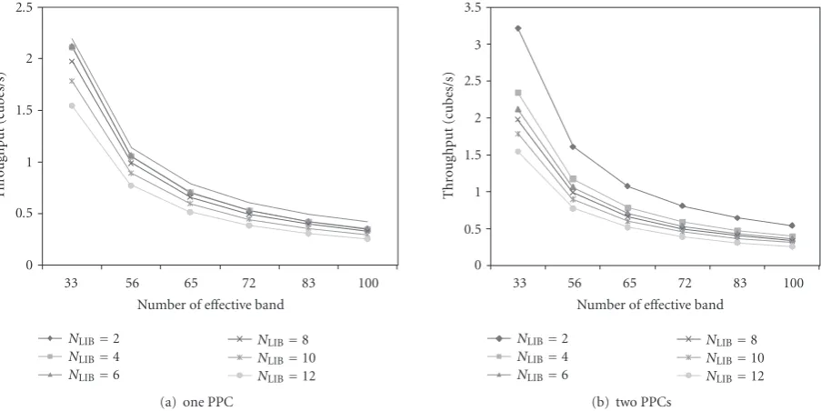
Figure 18shows the throughput in terms of the number
of effective bands and libraries, where one PPC or two
are used. In the fastest case, the throughput is 2.1099 or 3.2196. However, when the number of bands and libraries is increased, the advantage of two PPCs disappears since the
Preprocessing
Interconnection network
PE0
PE1
PE2
PE3
Stage A
Stage B
Stage A
Stage B
Stage A
Stage B
Stage A
Stage B
Interconnection network
Post-processing Refined
library Refined
library
Refined library
Refined library Sample Initial
Sample Initial
Sample Initial
Sample Initial
Figure14: Block diagram in multiple data partitioning without separated library.
Table1: Throughput comparison.
Type Resolution Used bands Second/cube
Estlick et al. [11] Wildstar (Vertex 1000) 614×512 10 0.41
Moigne et al. [8] SRC-6E (XC2V8000) 217×512 192 1.47
Du and Qi [10] Pilchard (Vertex1000E) 614×512 50 500
Single PE (Proposed) Xilinx Vertex-II pro 614×512 56 0.9
Multiple PE (Proposed) Xilinx Vertex-II pro 614×512 56 0.14
Preprocessing
Interconnection network
PE0
PE1
PE2
PE3
Stage A
Stage A
Stage A
Stage A
Interconnection network
Post-processing Refined
library Sample Initial Target
Refined library Sample Initial Target
Refined library Sample Initial Target
Refined library Sample Initial Target
Refined library Sample Initial
Stage B
PPC
FU
s
Basic
sp
2
4
5
+
+ +
1
clk clk
2
0
rd_en1
FU0
1
Accumulator
0
Accumulator
0
Accumulator
clk
BUFSP
Bank 0 Bank 1
BUFtg
clk
tg
FU3
BUFbk
clk bk
library
FU 0
rd_en0
Accumulator
0
Accumulator
clk
rd_en2
Accumulator
en_tg
en_bk
Post-processing
PPC
library
0
abs()
BUS Bank 0
Bank 1
BUFTG
Bank 0 Bank 1 Bank 2
FU
BUS1
rd_en0
Refined
BUFLIB
rd_en1
rd_en2
0
clk
0 clk
library
Refined
Preprocessing
bufi
clkw clkr
clkw clkr
clkw clkr
tk
rk libi j
2’s complement
clkL clks
enp enp
enc enc
Figure16: Illustration of a block diagram of a functional unit.
Tcube
TA
TB Tpixel
TF0
TF1
TP1
TF3
TF4
TP2a TP2b TF5 FU0
FU1 PPC1 FU3 FU4 PPC2 FU5
Figure17: Illustration of timing flow in the single-processing execution model.
of effective bands and libraries, but the complexity of PPC2 is invariant. Note that since our target architecture has the limited number of PPCs and the computation complexities
of PPC2 is much smaller than PPC1, we use one PPC for a
processing element.
4.2. Multiple-processing execution model
To enhance performance, the multiple-processing execution
model is introduced in Figure 19. The incoming image
0 0.5 1 1.5 2 2.5
Thr
o
ug
hput
(cubes/s)
33 56 65 72 83 100
Number of effective band
NLIB=2
NLIB=4
NLIB=6
NLIB=8
NLIB=10
NLIB=12 (a) one PPC
0 1 0.5 2 1.5 2.5 3 3.5
Thr
o
ug
hput
(cubes/s)
33 56 65 72 83 100
Number of effective band
NLIB=2
NLIB=4
NLIB=6
NLIB=8
NLIB=10
NLIB=12 (b) two PPCs
Figure 18: Illustration of throughput in terms of the number of effective bands and libraries in 614×512 resolution and 224 band
hyperspectral images.
Bank 0
FU0
FU0 FU1
FU0
FU0
FU1
FU1
FU1 FU3
FU3
FU3
FU3
FU5
FU5
FU5
FU5
FU4
FU4
FU4
FU4
PE0
Refined
library
Refined
library
Refined
library
Refined
library
PPC0
PPC2
Basic
library
PPC1
PPC3
Basic
library
Basic
library
Basic
library
Cube data
Bank 1
PE1
PE2
PE3
Figure19: Illustration of the overall diagram.
Each processing element uses one PPC for floating point operations.
Figure 20 illustrates the throughput in the multiple-processing execution model.
4.3. Throughput comparison and discussion
To minimize the effect of sequential operation, two kinds
of pipeline structures have been investigated. The functional units in Stage A can be parallel and the memory usage is to be optimized. We also implemented the floating point operation in the dedicated PPCs. To improve the execution
time, the multiple-processing execution model, whose design is scalable, has been proposed.
Table 1 compares the throughput with other FPGA designs. To compare our design with other designs, we chose the case of 56 bands and 4 libraries in the single-and multiple-processing element. The throughput is 0.9 or 0.14 seconds per cube. Estlick used the Annapolis Microsystems Wildstar PCI board which has three Xilinx Virtex 1000 FPGAs and a 500 MHz Pentium III workstation. However, for processing, one FPGA was used as 50 MHz
clock frequency for 614 ×512 images with 10 channels
0 2 4 6 8 10 12 14 16
Thr
o
ug
hput
(cubes/s)
33 56 65 72 83 100
Number of effective band
NLIB=2
NLIB=4
NLIB=6
NLIB=8
NLIB=10
NLIB=12
Figure 20: Illustration of throughput in the multiple-processing
execution model.
in SRC-6E, where 217× 512 resolution and a 192 band
image was used [8]. The SRC-6E architecture has two 1 GHz
Pentium microprocessors and two Xilinx Virtex II-6000-4 [9]. Du presented the parallel ICA algorithm in the Pilchard
board which has Xilinx Virtex V1000E FPGA, where 614×
512 resolution hyperspectral image and 50 selected bands were used, in which if the amount of weight vectors is four, the computational time requires 500 seconds [10].
5. CONCLUSION
A real-time target detection architecture for hyperspectral image processing is proposed in this paper. The architecture is based on a reduced complexity algorithm for high throughput applications. Multilevel pipelining of the archi-tecture enhances the overall throughput, and the archiarchi-tecture is scalable so that the execution speed improves with the number of processing elements. The proposed pipelining optimizes overall memory usage and eliminates the memory bottleneck. The proposed architecture has been designed and implemented in FPGA to verify the relationship between the hardware complexity and the execution throughput of the reduced complexity hyperspectral image processing.
ACKNOWLEDGMENTS
This research is supported by Foundation of Ubiquitous computing and Networking (UCN) Project, the Ministry of Information and Communication (MIC) 21st Century Frontier R\&D Program in Korea.
REFERENCES
[1] N. Keshava, “Distance metrics and band selection in hyper-spectral processing with applications to material identification and spectral libraries,”IEEE Transactions on Geoscience and Remote Sensing, vol. 42, no. 7, pp. 1552–1565, 2004.
[2] P. Bajcsy and P. Groves, “Methodology for hyperspectral band selection,”Photogrammetric Engineering and Remote Sensing, vol. 70, no. 7, pp. 793–802, 2004.
[3] K.-S. Park, S. Hong, and P. Park, “Spectral contents char-acterization for efficient image detection algorithm design,” in Proceedings of the 6th IEEE International Conference on Computer and Information Technology (CIT ’06), p. 137, Seoul, Korea, September 2006.
[4] W. E. Schaff, A. Copeland, M. Steffen, et al., “Real-time data processor for the COMPASS hyperspectral sensor system,” in Imaging Spectrometry IX, vol. 5159 ofProceedings of SPIE, pp. 1–13, San Diego, Calif, USA, August 2003.
[5] X. Liu, W. L. Smith, D. K. Zhou, and A. Larar, “Principal component-based radiative transfer model for hyperspectral sensors: theoretical concept,”Applied Optics, vol. 45, no. 1, pp. 201–209, 2006.
[6] M. R. Goupta and N. P. Jacobson, “Wavelet principal component analysis and its applocation to hyperspectral images,” inProceedings of the IEEE International Conference on Image Processing (ICIP ’06), pp. 1585–1588, Atlanta, Ga, USA, October 2006.
[7] S. Subramanian, N. Gat, A. Ratcliff, and M. Eismann, “Real-time hyperspectral data compression using principal component transform,” inProceedings of the AVIRIS AirBorne Geosciences Workshop, Pasadena, Calif, USA, February 2000. [8] J. Le Moigne, P.-S. Yeh, J. Joiner, et al., “Dimension reduction
of hyperspectral data on reconfigurable computers,” in Pro-ceedings of the 4th Annual Earth Science Technology Conference (ESTC ’04), Palo Alto, Calif, USA, June 2004.
[9] E. El-Araby, T. El-Ghazawi, J. Le Moigne, and K. Gaj, “Wavelet spectral dimension reduction of hyperspectral imagery on a reconfigurable computer,” in Proceedings of the IEEE International Conference on Field-Programmable Technology (FPT ’04), pp. 399–402, Brisbane, Australia, December 2004. [10] H. Du and H. Qi, “A reconfigurable FPGA system for
parallel independent component analysis,”EURASIP Journal on Embedded Systems, vol. 2006, Article ID 23025, 12 pages, 2006.
[11] M. Estlick, M. Leeser, J. Theiler, and J. J. Szymanski, “Algorithmic transformations in the implementation of K-means clustering on reconfigurable hardware,” inProceedings of the 9th ACM/SIGDA International Sysmposium on Field Pro-grammable Gate Arrays (FPGA ’01), pp. 103–110, Monterrey, Calif, USA, February 2001.
[12] M. Leeser, P. Belanovic, M. Estlick, M. Gokhale, J. J. Szy-manski, and J. Theiler, “Applying reconfigurable hardware to the analysis of multispectral and hyperspectral imagery,” in Imaging Spectrometry VII, vol. 4480 ofProceedings of SPIE, pp. 100–107, San Diego, Calif, USA, August 2001.
[13] G. A. Shaw and H.-H. K. Burke, “Spectral imaging for remote sensing,”Lincoln Laboratory Journal, vol. 14, no. 1, pp. 3–28, 2003.
[14] M. L. Nischan, R. M. Joseph, J. C. Libby, and J. P. Kerekes, “Active spectral imaging,”Lincoln Laboratory Journal, vol. 14, no. 1, pp. 131–144, 2003.
[15] M. K. Griffin and H.-H. K. Burke, “Compensation of hyperspectral data for atmospheric effect,”Lincoln Laboratory Journal, vol. 14, no. 1, pp. 29–54, 2003.
[17] B.-C. Gao, M. J. Montes, Z. Ahmad, and C. O. Davis, “Atmospheric correction algorithm for hyperspectral remote sensing of ocean color from space,”Applied Optics, vol. 39, no. 6, pp. 887–896, 2000.
[18] G. Girouard, A. Bannari, A. Harti, and A. Desrochers, “Validated spectral angle mapper algorithm for geological mapping: comparative study between quickbird and landsat-tm,” in Proceedings of the 20th International Society for Photogrammetry and Remote Sensing Congress (ISPRS ’04), pp. 599–605, Istanbul, Turkey, July 2004.