Removing Impulse Bursts from Images
by Training-Based Filtering
Pertti Koivisto
Department of Mathematics, Statistics, and Philosophy, University of Tampere, Finland Institute of Signal Processing, Tampere University of Technology, Tampere, Finland Email:[email protected]
Jaakko Astola
Institute of Signal Processing, Tampere University of Technology, Tampere, Finland Email:[email protected]
Vladimir Lukin
Department of Receivers, Transmitters, and Signal Processing, National Aerospace University (Kharkov Aviation Institute), Kharkov, Ukraine
Email:[email protected] Vladimir Melnik
Institute of Signal Processing, Tampere University of Technology, Tampere, Finland Email:[email protected]
Oleg Tsymbal
Department of Receivers, Transmitters, and Signal Processing, National Aerospace University (Kharkov Aviation Institute), Kharkov, Ukraine
Email:[email protected]
Received 18 March 2002 and in revised form 15 September 2002
The characteristics of impulse bursts in remote sensing images are analyzed and a model for this noise is proposed. The model also takes into consideration other noise types, for example, the multiplicative noise present in radar images. As a case study, soft morphological filters utilizing a training-based optimization scheme are used for the noise removal. Different approaches for the training are discussed. It is shown that these techniques can provide an effective removal of impulse bursts. At the same time, other noise types in images, for example, the multiplicative noise, can be suppressed without compromising good edge and detail preservation. Numerical simulation results, as well as examples of real remote sensing images, are presented.
Keywords and phrases:impulse burst removal, burst model, soft morphological filters, training-based optimization.
1. INTRODUCTION
Remote sensing images are usually formed on board an air-craft or spaceborne carrier where sensors and primary sig-nal processing devices are installed [1]. Then, the images are transferred to one or a few on-land remote sensing data-processing centers, where they are subject to visualization, analysis, filtering, interpretation, and so forth. For transfer-ring the remote sensing data, the standard or special com-munication channels are used and, since images are often en-coded and then deen-coded, impulsive noise may be observed in images [2].
In many practical situations, the probability of spikes is low and two or more neighboring pixels are very seldom corrupted by impulsive noise. In other words, the spikes pos-sess an approximately spatially invariant characteristic. Many efficient and robust filtering algorithms have been already proposed to remove spikes that fulfill the aforementioned model assumptions [3,4,5]. However, these assumptions are not valid in some practical situations.
(a) (b) (c) (d)
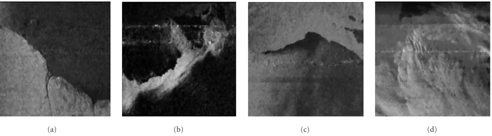
Figure1: Four 192×192 parts of the original satellite images. Images (a), (b), and (c) are radar images and image (d) is an optical image.
intensive that it corrupts several consecutive image pixels in one or more rows following each other. (In this paper, we as-sume that images are transferred rowwise. Naturally, similar effects can also be observed and methods similar to those ex-amined in this paper can be applied if images are transferred columnwise.) Such situations may happen if the receiver put and circuitry are not well protected against intensive in-terference or if in the neighborhood of the remote sensing data processing center, there are some electromagnetic wave irradiation sources operating in the frequency band which overlaps with the communication channel waveband.
Real life illustrations of what happens in this case with satellite images are presented in Figure 1. As can be seen, different amounts of horizontal impulse bursts appear in these images. This kind of bursts appearing as line-type noise considerably decrease the image quality. Hence, these bursts must be removed. This is, however, not a typical and easy task for the majority of commonly used filters.
It may seem that impulse bursts and multiplicative noise can be simultaneously removed by some robust scanning window filter. However, experiments show that such scan-ning window filters do not produce good results. The robust filters (e.g., the median filter) remove impulse bursts but at the same time they usually destroy details, small size objects, and texture too heavily. Other filters, for example, the center-weighted median and the modified sigma filter that was in-troduced [7] to filter images that are corrupted both by mul-tiplicative and by impulsive noise, are not robust enough and thus a lot of impulse bursts may remain in the images after the filtering.
Another possibility might be first to detect the pixels cor-rupted by impulse bursts and then to replace the correspond-ing values by new values, usually by takcorrespond-ing in some way into account the neighboring pixel values for which the bursts have not been detected. However, in general, spike detection methods (e.g., [8,9]) do not perform well in this task. The reason why these methods fail is that they have been designed to detect either isolated impulses or bursts whose character-istics differ from the characteristics of the considered impulse bursts.
One more possibility is to utilize training-based filter design. For example, Koivisto et al. [10] have shown that
training-based optimized soft morphological filters are able to remove line-type noise efficiently. The designed filters could also remove line-type noise with horizontal or almost horizontal orientations. As this noise in a certain sense cor-responds to the impulse bursts that we are considering, it is reasonable to expect that soft morphological filters being trained for the removal of impulse bursts are able to perform well for image recovery in our case.
There are also some differences between the task consid-ered here and the design task studied by Koivisto et al. in their paper. First, the impulse bursts differ from the line-type noise since the former one has more complicated and random be-havior. Second, besides impulse bursts, the remote sensing images usually contain other types of noise as well. For in-stance, the radar images are characterized by the presence of multiplicative noise [4]. Hence, the training task is now much more complicated.
In this paper, we analyze the properties of impulse bursts in remote sensing images and propose a model for this noise. The model also takes into consideration other noise types present in images. This model is then used in the forma-tion of the training images used in the optimizaforma-tion of the soft morphological filters. In addition, different approaches for the training and filtering are discussed. Finally, numeri-cal simulation results as well as test image and real remote sensing image examples are presented.
2. IMPULSE BURSTS IN REMOTE SENSING IMAGES
To get an idea what the impulse bursts are, we first an-alyze some real remote sensing images. The images for which the impulse bursts are observed are transferred from such low altitude satellites as NOAA (usually two satel-lites are operating with carrier frequencies 137.5 MHz and 137.62 MHz), Meteor (137.85 MHz), Sich (137.4 MHz), and Okean (137.4 MHz). The probability of the impulse bursts in the received data was the largest for the descending parts of the satellite orbits (just before the satellites escape under the horizon).
0 50 100 150 200 250
Pixel location
Pix
el
value
Figure2: Row 98 in the image inFigure 1a.
is slightly smaller. All aforementioned satellites use, as one possible mode, the AM APT (automatic picture transmis-sion) format, for which the image information is contained in the amplitude modulation of 2400 Hz subcarrier. More detailed information can be found, for example, in [6].
For the reception of the signals carrying the image infor-mation, we have to use a converter for the microwave fre-quency with an input at 137 MHz. The received images can then be decoded, and the resulting bitmap images (in some cases, these are images formed in different wavebands includ-ing radar, visible optical, and infrared) can be stored, pro-cessed, and visualized by standard programs. The modula-tion and decoding modes are not very well protected against interference that may be present in the 137 MHz band. This interference can radically degrade the structure of the re-ceived signal. Hence, decoding errors appearing as impulse bursts may occur.
Four 192×192 parts of real satellite images are presented inFigure 1. As can be seen, several fragments in many rows are corrupted by impulse bursts, and the lengths of such frag-ments are rather different. Sometimes such fragments occur in two consecutive rows. It can also be observed that in some pixels of the considered fragments, the values are maximal (i.e., 255 in the 8-bit representation used) while most of the pixel values in the fragments differ from 255 but still remain “impulsive” with respect to the values that can be predicted for the satellite images from their local analysis. Similar ef-fects can also be observed with the minimal value (i.e., 0).
3. PROPERTIES OF IMPULSE BURSTS
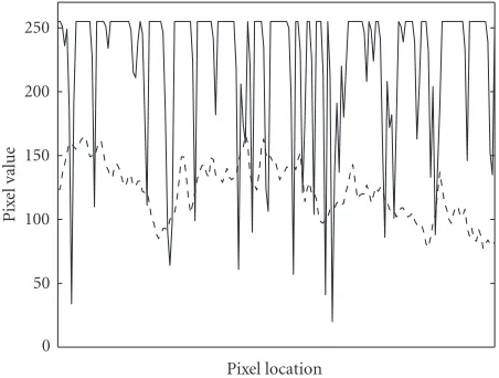
In order to make an adequate model for a test remote sens-ing image, we studied the properties of the real satellite im-ages in detail. More precisely, the statistical characteristics of impulse bursts and the signal sample behavior were carefully studied row by row for the rows containing bursts. Examples of such rows are given in Figures2and3. As can be seen, row 98 inFigure 2contains two short-time impulse bursts located at the right part of the row. The presence of multiplicative
0 50 100 150 200 250
Pixel location
Pix
el
value
Figure 3: Rows 167 (dashed) and 168 (solid) in the image in Figure 1d.
noise in this radar image is also clearly seen. For compari-son, row 168 in Figure 3is practically fully corrupted by a long-term burst while row 167 inFigure 3does not contain impulse bursts and shows a typical cross section of the op-tical image in Figure 1d. Altogether, more than 50 impulse bursts taken from the images inFigure 1were analyzed.
It was found out that the means of the impulse bursts were usually larger than the mean of the pixels not corrupted by bursts. Visually, this means that the observed impulse bursts mainly appear as light horizontal distortions that may corrupt even two or more neighboring rows. Usually, the mean of the values of an impulse burst is larger than 160 but smaller than 190.
Most impulse bursts also contain a periodical (quasisinu-soidal) component and a random noise component. Using spectral analysis of short-term time series [11], we found out that one harmonic component was practically always much larger than the other harmonic components. Hence, the lat-ter ones can be considered as noise. Aflat-ter this, it was possible to estimate the amplitude and the normalized circular fre-quency of the dominant sinusoidal component. According to our experiments, the amplitude was from 50 to 90 while the circular frequency varied from 0.3 to 1.0. The phase of the dominant sinusoidal component seemed to be random.
When the values for the amplitude and frequency had been estimated, it was possible to evaluate the power of the other spectral components and, using Parseval’s theorem [11], to estimate the variance (or the standard deviation) of the random noise component. The estimates obtained for the standard deviation were from 22 to 40. It was also possible to consider the noise component as consisting of independent and identically distributed (i.i.d.) random variables.
Finally, the probability that a pixel belongs to an impulse burst was estimated. For the considered images, this prob-ability was from 0.01 to 0.05. The length of the bursts was random. In the considered images, the shortest bursts were only a few pixels long while the longest ones contained hun-dreds of pixels.
4. NOISE MODEL
All aforementioned properties of impulse bursts have been taken into account when generating the noise model for the test images. As a case study, the model is gener-ated for side-look aperture radar (SLAR) images. Hence, the images are supposed to contain multiplicative noise with Gaussian probability density function with 1.0 as the mean [1, 4]. Empirical tests confirm this assumption for the test images. In our cases, the estimated relative vari-ance σ2
µ of the multiplicative noise varied from 0.015 to 0.055. Since the images are transferred as one-dimensional arrays, the noise model is also presented for one-dimensional array. More precisely, our noise model is the following.
First, a Markov chain with two states is used to determine which samples (fragments) belong to impulse bursts [12]. The transition probability from “no-burst state” to “burst state” is p, and the transition probability from “burst state” to “no-burst state” isq. The values of these variables should be based on the estimated percentage of the pixels corrupted by impulse bursts.
If a sample does not belong to an impulse burst, then it is corrupted by the aforementioned multiplicative noise in the usual way. That is, the (corrupted) sample valueXjis given by
Xj=µjXj, (1)
where Xj is the corresponding value of the original signal andµjis the multiplicative noise component having relative varianceσ2
µ (and mean equal to 1.0). If we do not want to add multiplicative noise (e.g., the image is a satellite image that is already corrupted by multiplicative noise), we can set
σ2 µ=0.
On the other hand, if the jth sample belongs to thekth impulse burst, then the (corrupted) sample valueXj is ob-tained using the formula
Xj=roundαk+βksinj−lkωk+ϕk+ξj, (2)
wherelkdenotes the index of the leftmost sample in the burst (i.e., the starting index of the burst),αkis the average level of the impulsive noise in the burst,βk andωk are the am-plitude and the circular frequency of the harmonic compo-nent of the burst, respectively, ϕk denotes the phase of the harmonic component of the burst, andξjis the fluctuating noise component of the burst. The parameters αk, βk,ωk, andϕkare random variables with uniform distribution from
the intervals1Ꮽ ⊆[0,255],Ꮾ ⊆[0,255],ᏻ⊆[0,2π[, and
]−π, π], respectively. The noise componentξjis a random variable with Gaussian probability density function with zero mean and standard deviationσk, whereσkis a random vari-able with uniform distribution from the interval⊆[0,∞[. Rounding is to the nearest nonnegative integer less than or equal to 255.
Hence, the parametersαk,βk,ωk,ϕk, andσkchange from burst to burst but are common to all pixels in some burst. The parameterξjvaries from pixel to pixel. The parameters are modeled as random variables to simulate the random be-havior of the impulse bursts in the real satellite images.
In order to apply the noise model, we thus need the val-ues for the parameters pandqthat control the amount and length of the bursts, and the limits for the intervalsᏭ,Ꮾ,ᏻ, andthat affect the behavior of a single burst. If our image is artificial, then the relative varianceσ2
µof the multiplicative noise component is also needed.
When forming the test images in this paper (seeSection 5.2), the parameter values used werep=0.0007,q=0.011,
Ꮽ = [160,190],Ꮾ = [50,90], ᏻ = [0.3,1.0], and =
[22,40]. The relative varianceσ2
µ for the multiplicative noise in the artificial images was 0.02. Naturally, the parameter val-ues given here are not the only possibilities but other slightly different parameter values could be used as well. However, the chosen values are suitable to our purposes, and based on our experiments, the values given here may also be used even in quite different situations.
As the selection of the parameter values was based on a detailed analysis of the real remote sensing images, the val-ues can also be used as a starting point for the selection of the parameter values in other cases. That is, when choosing parameter values for some other case, we can start from the values given here, and if we want any changes to the noise characteristics, we can modify the values in a straightforward way to suit other purposes.
For example, if we want less bursts, we can choose a smaller value for p, and if we want to increase the number of bursts, we can increase the value of p. Likewise, smaller values forqimply longer bursts and larger values forqimply shorter bursts. The overall level of the multiplicative noise can be controlled by decreasing or increasing the relative varianceσ2
µ, and if we want to decrease or increase the aver-age level of the impulse bursts we can, respectively, either de-crease or inde-crease the limits of the intervalᏭ. Besides, the in-tervalᏭcan also be shortened or lengthened, which causes, respectively, less or more variations in the average levels of separate bursts.
Decrease in the limits for the amplitude of the harmonic component (i.e., in the intervalᏮ) implies less variation in a single burst and, conversely, increase implies more variation. The same usually also holds for the limits of the frequency of the harmonic component (i.e., for the intervalᏻ) although the periodical nature of the harmonic component may
some-1Sometimes the half-open intervals [a, b[ and ]a, b] are also denoted by
times cause odd effects (i.e., aliasing). As above, shorter or longer intervals mean, respectively, less or more variations in the properties of separate bursts. Finally, the weight of the noise component can be controlled by decreasing or increas-ing the limits for the standard deviationσk(i.e., for the inter-val).
Besides variations in the parameter values, other modi-fications in the noise model are possible as well. For exam-ple, instead of multiplicative noise typical for the radar im-ages, additive Gaussian noise typical for optical images can be used.
5. TRAINING-BASED FILTERING
In noise removal applications, the task in the training-based design method is to find a filter that transforms the noisy data as close as possible to the desired ideal data. The obtained fil-ter can then be applied to other situations with similar char-acteristics as well. Several error criteria can be used and the training data can be either natural or artificially generated (see, e.g., [13,14,15]).
The filter is usually sought from a specified filter class to keep the optimization reasonably simple. In this paper, we utilize the class of soft morphological filters. This class was selected since we know that the training-based optimized soft morphological filters are able to remove line-type noise effi -ciently [10]. Moreover, although the optimization of the soft morphological filters is not at all trivial, it can be done in a reasonable time.
5.1. Soft morphological filters
Soft morphological filters form a class of stack filters and were introduced to improve the behavior of standard flat morphological filters in noisy conditions [16]. They have many desirable properties, for example, they can be designed to preserve details well [17]. In addition, they are suitable for impulsive or heavy-tailed noise.
The two basic soft morphological operations are soft ero-sion and soft dilation. Based on them, compound operations can be defined in the usual way.
Definition 5.1. The structuring system [B, A, r] consists of three parameters, finite setsAandB,A ⊆ B = ∅, ofZ2,
and an integerrsatisfying 1≤r≤max{1,|B\A|}. The setB is called thestructuring set,Aits (hard)center,B\Aits (soft) boundary, andrtheorder indexof its center or therepetition parameter.
Thetranslated setTx, where the setT ⊂Z2is translated
byx,x∈Z2, is defined byT
x= {x+t:t∈T}. Thesymmetric set ofTis the setTs = {−t :t∈T}. Amultisetis a collec-tion of objects, where the repeticollec-tion of objects is allowed. For example,{1,1,1,2,3,3} = {3♦1,2,2♦3}is a multiset.
Soft morphological operations transform a signal X : Z2→Rto another signal by the following rules.
Definition 5.2. Soft erosionof X by the structuring system [B, A, r] is denoted byX [B, A, r] and is defined byX
[B, A, r](x)=therth smallest value of the multiset{r♦X(a) :
a∈Ax} ∪ {X(b) :b∈(B\A)x}for allx∈Z2.
Definition 5.3. Soft dilationofX by the structuring system [B, A, r] is denoted byX⊕[B, A, r] and is defined byX⊕
[B, A, r](x)=therth largest value of the multiset{r♦X(a) :
a∈Ax} ∪ {X(b) :b∈(B\A)x}for allx∈Z2.
Afinite compositionof lengthpof basic soft morpholog-ical operations is given by
always mean by the term composite filter a finite composi-tion of basic soft morphological filters.Soft openingandsoft closingare special cases of composite soft operations. Then, we have a soft erosion-dilation (opening) or dilation-erosion (closing) pair with equal order index values and symmetric structuring sets. If all the structuring setsBiare subsets of the
n×mrectangle, thennandm(orn×m) are called theoverall dimensionsof the corresponding composite filter.
The detail preservation ability, as well as the noise re-moval capability of a soft morphological filter, depends on the size and shape of its structuring set and on the value of its order index.
5.2. Training images
Although there are no analytical criteria for deciding which soft morphological operation (and with which parameters) is the best for some situation, a suitable operation sequence and its parameters can be found using supervised learning methods, for example, simulated annealing and genetic al-gorithms [10]. Of course, some training set, for which the desired output is known, is needed.
In this paper, we use both artificial images and real satel-lite images as training images. An artificial test image of size 256×256 and its three noisy counterparts are presented in Figure 4. The image inFigure 4ais the noise-free test image, the image inFigure 4b is corrupted by multiplicative noise only, the image inFigure 4cis corrupted by impulse bursts only, and the image inFigure 4dis corrupted both by multi-plicative noise and by impulse bursts. As can be seen, the test image contains homogeneous regions, large size objects with different shapes, and small size objects also having different shapes, contrasts, and orientations. To simulate the presence of texture in real satellite images, the test image also con-tains four textural regions with different spatial correlation and statistical properties.
Our desire was also to check whether the soft morpholog-ical filters destroy many details while removing the impulse bursts. By comparing the images in Figures1and4, we can see that the structure and general properties of the images are similar enough also for this purpose.
(a) (b) (c) (d)
Figure4: The artificial test images used. (a) The noise-free (i.e., uncorrupted) image. The original image corrupted (b) by multiplicative noise, (c) by impulse bursts, and (d) both by multiplicative noise and by impulse bursts.
(a) (b) (c) (d)
Figure5: Four 192×192 parts of the original satellite images.
(a) (b) (c) (d)
Figure6: The images inFigure 5corrupted by impulse bursts.
size 192×192 (Figure 5) and their counterparts corrupted by bursts (Figure 6) are represented. The latter images are ob-tained by corrupting the original images by impulse bursts. A restriction concerning the satellite training images is that, unfortunately, we do not have noise-free test images but all images are corrupted by multiplicative noise. Hence, these images can be used if we try to remove only impulse bursts but they cannot be used if we also try to remove multiplica-tive noise at the same time.
When forming the test images, the parameter values used in the noise model for the impulse bursts wereᏭ =
[160,190],Ꮾ = [50,90],ᏻ = [0.3,1.0], and = [22,40]. The parameter values controlling the amount and length of the impulse bursts were p =0.0007 andq = 0.011 for the test images that contained bursts and p = 0 andq = 1 for the test image inFigure 4b(in which case no bursts ap-peared). The relative varianceσ2
other test images (in which cases no multiplicative noise was added).
For technical reasons, we made one technical modifica-tion to the noise model when forming the test images in this paper. Namely, the satellite images are often transferred as a group where several images are considered to be one larger image. Thus, although it may seem that one burst continues from the right end of a line to the beginning of the next line, it may be that in reality one burst does not continue from one line to another but, in fact, we have two separate bursts. Hence, we have supposed that if a burst continues from one line to another, the values of the parametersαk, βk,ωk,ϕk, andσkcommon to a burst are also changed.
5.3. Optimization
The optimization methods given in Koivisto et al. [10] allow one to handle impulse bursts in several ways. Basically, there are two different possibilities. We can either try to remove both the impulse bursts and the multiplicative noise at the same time or concentrate to remove only the impulse burst and disregard the multiplicative noise. The latter approach may be useful, for example, if the amount of the multiplica-tive noise is low.
If we try to remove both the impulse bursts and the mul-tiplicative noise, a straightforward solution is to use a source image that contains both impulse bursts and multiplicative noise and a target image that is free of the bursts and of the multiplicative noise. A suitable training image pair is thus, for example, the image inFigure 4das the source image and the image inFigure 4aas the target image.
A more refined solution is to employ structural con-straints, in which case the target image is again the noise-free image but the source image is the image corrupted by mul-tiplicative noise only. Thus, a suitable training image pair is, for example, the image inFigure 4bas the source image and the image inFigure 4aas the target image. The impulse bursts are presented as constraints and an optimal filter is sought provided that the impulse bursts are removed (totally or at least to some extent). This method is more flexible than the straightforward one since we can now control to what extent the impulse bursts should be removed. Unfortunately, this also means that the method needs more tuning, that is, there are more parameters for the user.
Both of the aforementioned methods need a noise-free training image as the target image. Since the real satellite im-ages are in any case corrupted by multiplicative noise, they cannot be used. Unfortunately, only artificial training images can thus be used with these methods.
The other possibility is to optimize the soft morpholog-ical operations to remove only impulse bursts (and to pre-serve details). At the second stage, multiplicative noise can then be suppressed by some conventional technique suited for this purpose, for example, the local statistic Lee filter, the sigma filter, or a combination of them [4,18,19,20,21]. In general, the selection of a suitable filter for the postprocessing may depend on the task at hand. However, we can say that the local statistic Lee filter [18] and the locally adaptive schemes
[21], where the local statistic Lee filter is applied only to tex-ture regions, seem to preserve edges, details, and textex-ture fea-tures well.
Again, we can use the straightforward solution or we can utilize the structural constraints. In the first case, the training image pair consists of an image corrupted by impulse bursts as the source image and the same image without bursts as the target image. In the latter case, we use the same image as the source and target image. In theory, any images can be used as training images, but in practice, the training images should be such that they incite the filters to preserve details well. The impulse removal is namely not the only goal but the optimal filter should also preserve details well, that is, it is very easy to remove all bursts if we may destroy all details.
Suitable artificial training image pairs in the straightfor-ward solution are thus, for example, the test image corrupted only by the impulse bursts (Figure 4c) as the source image and the noise-free image inFigure 4aas the target image, or the test image corrupted by impulse bursts and multiplica-tive noise (Figure 4d) as the source image and the test im-age corrupted by multiplicative noise (Figure 4b) as the tar-get image. The motivation for the first training image pair is that if we are trying to preserve details and to remove im-pulse bursts only, then the test images should not contain any other type of noise. The motivation for the latter case is that since impulse bursts usually appear together with multiplica-tive noise, bursts should also be removed assuming that the images contain multiplicative noise.
The last comment also motivates the use of real satel-lite images as training images. That is, if we have satelsatel-lite images that are not corrupted by impulse bursts, they can also be used as training images. Suitable training image pairs are thus also the test images corrupted by impulse bursts (Figure 6) as the source images together with the correspond-ing original satellite images inFigure 5as the target images.
If we utilize structural constraints, all aforementioned images that do not contain impulse bursts can be used as the source/target image. Since our aim under the structural constraints is good detail preservation, it may, however, be unreasonable to use test images corrupted heavily by multi-plicative noise as the source/target image.
As the error criterion, it is possible to use any criterion that can be calculated using two images as parameters. In this paper, we have used the mean absolute error (MAE) and the mean square error (MSE). Sometimes, the peak signal-to-noise ratio
PSNR=10 log102552/MSE (4) is also calculated for comparison purposes.
than large enough to prevent overlearning. The experimental results given inSection 6demonstrate that the designed filter can solve possible new situations in a satisfactory manner.
6. EXPERIMENTAL RESULTS
First, we should note that in this paper we call the best filters obtained by our method optimal although there is no abso-lute guarantee that they are globally optimal.
6.1. Test case
The experimental tests reported in this paper are based on the following test cases. The training image pairs are the ones discussed in Sections5.2and5.3. The application images are the ones shown inFigure 1. The optical image inFigure 1dis included for comparison purposes. In each test, an optimal composite operation of length two was sought with overall dimensions 3×3, 3×5 (i.e., 3 columns and 5 rows), and 5×5. Both nonsymmetric and symmetric structuring sets were used. Note that, in this section, “symmetric structuring set” means that the structuring set is symmetric with respect to the x- and y-axes, not with respect to the origin as the symmetric set was defined inSection 5.1.
The length two was selected since the noisy images con-tain both positive and negative impulsive noise and a single basic soft operation is not able to remove two-sided noise. On the other hand, as the experiments show, two consecu-tive soft operations are already powerful enough for our pur-poses.
6.2. Basic results
When the 3×3 window was used, the optimal filters were not able to remove the impulse bursts sufficiently. On the other hand, the filters optimal inside the 3×5 and 5×5 windows were already able to remove almost all of the bursts. Hence, the quality of these filters depends on their ability to remove multiplicative noise and preserve details. As the 3×5 case is a subcase of the 5×5 case, an optimal composite filter with the overall dimensions 5×5 naturally outperforms the one with the overall dimensions 3×5. On the other hand, the optimization is easier with the overall dimensions 3×5. In practice, the results with the overall dimensions 5×5 are only slightly better than those with the overall dimensions 3×5, and the optimization using the overall dimensions 3×5 is much easier than the optimization using the overall dimen-sions 5×5. Hence, in our examples, it is not reasonable to use the overall dimensions 5×5 but the examples are based mostly on the 3×5 case.
The results obtained using symmetric structuring sets were usually not as good as those which were achieved with-out any restrictions (i.e., nonsymmetric structuring sets were also allowed). However, the differences were usually small. The PSNRs obtained by the symmetric structuring systems were usually only 0.1 dB less than the corresponding values for the nonsymmetric case (see Tables 1 and2). Since the noise process is symmetric and we cannot make any assump-tions about the structure of the application images, it is in any case safe to use symmetric structuring sets. Thus, most
of the examples in this paper are also based on the symmet-ric structuring sets.
The results are at least in the quantitative sense better when using nonsymmetric structuring sets because in soft morphological filtering, the ratio r/|B\A|(i.e., the value of the order index divided by the size of the soft bound-ary) plays a very important role [10], and with nonsymmet-ric structuring sets, we have much more possibilities to tune this ratio to be suitable for the optimization task in ques-tion, especially when the size of the soft boundary is small. An undesirable side effect is that sometimes this may also lead to slight overlearning. This ratio has much to do with the breakdown point of a basic soft morphological filter [22], and the ratio controls the amount of the impulsive noise that our filters can remove, so that the lower the value for the ratio is, the more impulses will be removed. The optimal value for the ratio is then the highest value such that almost all impulse bursts will be removed.
The optimal filter sequence was usually a soft erosion fol-lowed by a soft dilation, as can also be seen from the optimal sequences in Figures7,11, and12. This combination is natu-ral since the impulse bursts were mostly positive. The results obtained by the optimal soft openings were usually almost as good as those obtained using the optimal composite soft op-erations of length two. This is important since the optimiza-tion of soft openings is much easier than the optimizaoptimiza-tion of the composite soft operations of length two.
The error criterion (i.e., the MAE or the MSE) did not seem to have crucial effect in the optimization. The filters optimized under the MSE produced usually visually better results although, in general, the differences were small.
When comparing the optimization schemes, we noticed that by selecting the details in the optimization schemes in a suitable manner, all schemes were able to produce good re-sults. The suitability of some optimization scheme thus de-pends much on whether we want to emphasize the burst moval capability or the detail preservation ability of the re-sulting filter.
6.3. Bursts and multiplicative noise
In this section, we study the experiments where we remove both impulse bursts and multiplicative noise at the same time. Both the straightforward optimization and the struc-tural constraints are employed.
Table1: The MSEs (and the corresponding PSNRs) between the target training images and the source training images filtered by the optimal filters with the overall dimensions 3×5 and the symmetric and nonsymmetric structuring sets. The filters were trained to remove impulse bursts only.
MSE
Source image Target image Original Symmetric No restrictions
Figure 4c Figure 4a 483.4 85.2 80.6 Figure 4d Figure 4b 490.8 147.9 145.6 Figure 6a Figure 5a 1059.4 42.4 40.3 Figure 6b Figure 5b 1069.7 43.7 43.6 Figure 6c Figure 5c 460.7 61.5 61.5 Figure 6d Figure 5d 860.8 122.0 121.5
PSNR
Source image Target image Original Symmetric No restrictions
Figure 4c Figure 4a 21.3 28.8 29.1 Figure 4d Figure 4b 21.2 26.4 26.5 Figure 6a Figure 5a 17.9 31.9 32.0 Figure 6b Figure 5b 17.8 31.7 31.7 Figure 6c Figure 5c 21.5 30.2 30.2 Figure 6d Figure 5d 18.8 27.3 27.3
Table2: The MSEs (and the corresponding PSNRs) between the target training image and the source training image filtered by the optimal filters with the overall dimensions 3×5 and the symmetric and nonsymmetric structuring sets. The filters were trained to remove both impulse bursts and multiplicative noise. Note that different methods utilize different source images.
MSE
Optimization method Original Symmetric No restrictions
Straightforward optimization 745.5 190.0 187.7
Structural constraints 274.0 162.3 160.6
PSNR
Optimization method Original Symmetric No restrictions
Straightforward optimization 19.4 25.3 25.4
Structural constraints 23.8 26.0 26.1
Figure 8a shows the resulting image when the noisy image in Figure 4d is filtered using the optimal filter in Figure 7a. As can be seen, the image inFigure 8ais a little blurred and some small details are lost. However, practically, all impulse bursts have disappeared and the texture as well as most of the details are preserved.
Figure 9illustrates what happens when the filter sequence in Figure 7a is applied to the real satellite images given in Figure 1. Again, almost all impulse bursts have disappeared and small distortion has appeared. It is also worth mention-ing that although the trainmention-ing image in our case study was based on radar images (i.e., multiplicative noise), the ob-tained optimal filter also works well with the optical image inFigure 9dthat was originally corrupted instead of multi-plicative noise by additive noise. Hence, the obtained filter can be applied to a variety of different satellite images.
When the structural constraints were used together with the requirement that all impulse bursts must be removed, the resulting images were somewhat blurred. Hence, if structural
constraints are used, it is advisable to allow that a small por-tion of impulse bursts may remain after the filtering. Nat-urally, the requirement to which extent the bursts must be removed can be used to control the detail preservation abil-ity and the impulse removal capabilabil-ity of the optimal filter in other ways as well.
Figure 7b shows the structuring systems of the opera-tion sequence optimized utilizing the structural constraints. Again, the sequence with symmetric structuring sets was found under the MSE and with the overall dimensions 3×5. The source image was the artificial test image corrupted by the multiplicative noise (Figure 4b) and the target image was the noise-free image in Figure 4a. The impulse bursts were presented as constraints and the optimal filter was sought provided that almost all (however, not all) of the impulse bursts are removed.
1. oper. (erosion)
2. oper. (dilation)
r=10 r=3 (a)
1. oper. (erosion)
2. oper. (dilation)
r=9 r=7 (b)
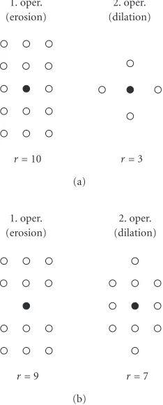
Figure7: The (symmetric) structuring systems of the soft opera-tion sequences optimized to remove both impulse bursts and mul-tiplicative noise utilizing (a) straightforward optimization and (b) structural constraints (• =the hard center=the origin,◦=the soft boundary, andr=the order index).
removal of multiplicative noise. Although the optimal struc-turing systems are not the same as those obtained using the straightforward optimization, they are, however, quite simi-lar. In both cases, the second operation focuses on the mul-tiplicative noise and the first operation is a soft erosion with large structuring set, which is suitable for the burst removal. Moreover, the ratios r/|B\A|do not differ much. For the structuring systems obtained using the straightforward op-timization, they are 0.71 and 0.75, and with the structural constraints, they are 0.75 and 0.7. Hence, both operation se-quences should perform much in the same way.
Figure 8bshows the image that is obtained by filtering the image corrupted by the impulse bursts and the multiplica-tive noise (Figure 4d) using the filter sequence inFigure 7b. As can be seen, the optimal filter removes bursts and mul-tiplicative noise well but at the same time some small, espe-cially horizontal, details are lost. When comparing the images in Figures8aand8b, we notice that the filter obtained using the structural constraints removes better impulse bursts than the filter obtained by the straightforward method. Unfortu-nately, at the same time, it also destroys more details.
As can be seen from the images inFigure 10, the afore-mentioned phenomenon also appears when the satellite
(a) (b)
Figure8: The artificial test image inFigure 4dfiltered by the op-timal symmetric composite soft operation of length two. The fil-ters were optimized to remove both impulse bursts and multiplica-tive noise using (a) straightforward optimization and (b) structural constraints.
images are filtered by the filter sequence in Figure 7b. That is, only few impulse bursts remain but some very small de-tails have disappeared. Again, the obtained filter also works well with the optical image inFigure 10d.
6.4. Burst removal
Next, we concentrate on the removal of the impulse bursts. In the tests, four satellite images and one artificial image (both with and without multiplicative noise) were used as the training images. Some of the optimal symmetric struc-turing systems with overall dimensions 3×5 found under the MSE are shown in Figures11and12. Again, the optimal filter sequences were soft erosions followed by soft dilations. The filters inFigure 11were optimized utilizing the satellite training images, and the filters in Figure 12were obtained using the artificial training images. The target images were thus the satellite images inFigure 5and the artificial images in Figures4aand4b, and the source images were the target images corrupted by impulse bursts, that is, the satellite im-ages inFigure 6and the artificial images in Figures4cand4d, respectively.
Although not identical, the optimal structuring systems are quite similar. They also have much in common with the optimal structuring systems in Section 6.3. Again, the first operation (soft erosion) is the one that removes the bursts. Moreover, the structuring systems of the first operation are nearly alike. The second operation (soft dilation) is in all cases very weak and its role is to remove the negative parts of the bursts and to correct the bias that the first operation causes.
(a) (b) (c) (d)
Figure9: The original satellite images inFigure 1filtered by the optimal symmetric composite soft operation of length two (seeFigure 7a) that was optimized using the straightforward optimization.
(a) (b) (c) (d)
Figure10: The original satellite images inFigure 1filtered by the optimal symmetric composite soft operation of length two (seeFigure 7b) that was optimized using the structural constraints.
reason is that a large structuring set means now less changes upwards. Hence, a large structuring set also produces better detail preservation which is useful when the training image contains a lot of texture.
In all cases, the optimal filters could remove impulse bursts with efficiency, as can also be seen from the MSE and PSNR values in Table 1. Since the amount of the bursts is about the same in all cases, the differences in the original er-rors are quite much explained by the fact that the general level of the background varies from image to image. That is, the darker the background is, the larger values for the MSE we have. The substantial improvement for the test im-ages in Figures5aand5bis explained by the smaller amount of texture in these images. The smallest improvement was achieved when the artificial images corrupted by the multi-plicative noise were used as the training images. Then, the target image contained so many “details” (i.e., details, tex-ture, and multiplicative noise) that the optimal filter was not anymore able to remove bursts with full efficiency. The re-sults obtained utilizing structural constraints where in coher-ence with the results reported here.
Visually, the differences between different schemes were again quite small. For comparison purposes,Figure 13shows
two images that are obtained by filtering the artificial test age corrupted both by the multiplicative noise and the im-pulse bursts (Figure 4d) using the found optimal filters. The image inFigure 13ais the result when the image inFigure 4d is filtered by the operation sequence inFigure 11a and the image inFigure 13bis the result when the same image is fil-tered by the operation sequence inFigure 12a. That is, the first filter was optimized with the satellite image inFigure 6a as the source image and the satellite image in Figure 5a as the target image, and the second filter was optimized with the artificial image inFigure 4cas the source image and the noise-free artificial image inFigure 4aas the target image.
1. oper. (erosion)
2. oper. (dilation)
r=8 r=4 (a)
1. oper. (erosion)
2. oper. (dilation)
r=9 r=10 (b)
1. oper. (erosion)
2. oper. (dilation)
r=9 r=14 (c)
1. oper. (erosion)
2. oper. (dilation)
r=8 r=14 (d)
Figure11: The (symmetric) structuring systems of the soft opera-tion sequences optimized using the satellite images in Figures (a)6a and5a, (b)6band5b, (c)6cand5c, (d)6dand5das the training images (• =the hard center=the origin,◦=the soft boundary, and
r=the order index).
1. oper. (erosion)
2. oper. (dilation)
r=7 r=10 (a)
1. oper. (erosion)
2. oper. (dilation)
r=11 r=14 (b)
Figure12: The (symmetric) structuring systems of the soft opera-tion sequences optimized using the artificial images in Figures (a) 4cand4a, and (b)4dand4bas the training images (• =the hard center=the origin,◦=the soft boundary, andr=the order index).
(a) (b)
Figure13: The artificial test image inFigure 4dfiltered by the op-timal symmetric composite soft operation of length two. The filters were optimized to remove impulse bursts only using (a) the satellite training images in Figures6aand5a, and (b) the artificial training images in Figures4cand4a.
Naturally, most of the multiplicative noise remains in the images but as we already noted, if there is a need, the multi-plicative noise can be removed by postprocessing filters. Ex-perimental tests show that with these images, a suitable post-processing filter can improve the PSNRs about 1.5 dB.
(a) (b) (c) (d)
Figure14: The original satellite images inFigure 1filtered by the optimal symmetric composite soft operation of length two (seeFigure 11a) that was optimized using the satellite images in Figures6aand5aas the training image pair.
method is applied to the real satellite images. The utilized operation sequence was the one shown inFigure 11a, that is, the one optimized using the satellite image inFigure 6aas the source image and the satellite image inFigure 5aas the target image. As can be seen, practically, all bursts have disappeared but most of the negative noise remains, which can be seen as black dots in the images. When compared to images in Fig-ures9and10, we can see that the results are quite similar. Less bursts and more details remain but, in contrast, the im-ages contain more black dots.
6.5. Comparison tests
We also compared the obtained filters to existing filters. The chosen comparison filters were the median filter, the center-weighted median (CWM) filter, and the Wilcoxon filter that are either robust or should perform otherwise efficiently in this kind of situations [3,5,23] (for the definition of the fil-ters, see, e.g., [3,5]). For all filters, different window sizes were tested. The quantitative results of the comparison are shown in Table 3. For the median filter and the CWM fil-ter with 3 as the cenfil-ter weight (CWM-3), the best results with respect to the MSE criterion were obtained using the 3×3 window. For the CWM filter with 5 as the center weight (CWM-5) and for the Wilcoxon filter, the best results were obtained using the 3×5 window.
The corresponding MSE and PSNR values between the image in Figure 4a and the image inFigure 4d filtered by the filters optimized to remove both the impulse bursts and the multiplicative noise are 187.7 and 25.4 for the operation sequence optimized using the straightforward optimization and 193.3 and 25.3 for the operation sequence optimized us-ing the structural constraints. When compared to the results shown inTable 3, we can see that the methods discussed in this paper clearly outperform the comparison filters. Visu-ally, the resulting images were in coherence with the quanti-tative results.
Finally, we compared our methods to methods where the idea is first to detect the corrupted pixels and then to replace the corresponding values by new values usually by taking, in some way, into account the neighboring pixel values for which the bursts have not been detected. However, for
ex-ample, the method proposed by Abreu et al. [8] did not de-tect impulse bursts satisfactorily and due to this, quite many bursts were remaining after the filtering. Moreover, since only the values of the detected samples are changed, most of the multiplicative noise remains in the image. Taken all to-gether, this results in MSE value 366.5 (PSNR 22.5 dB), which is even worse than that with the other comparison methods. We also tested the method of primary local recognition proposed by Dolia et al. [9]. The method was introduced to detect spikes in images corrupted by mixed multiplicative and impulsive noise. However, this method also failed and produced a quite low percentage of correctly detected spikes. We must admit that the burst detection methods may produce good results in some specific cases. Especially, if the amount of the bursts and other noise in the image is low, we can avoid unnecessary filtering if we first detect the bursts. This is also how the soft morphological filters work, that is, if the filter does not think that a sample is an impulse, then no changes, or at least only small changes, will be done. A future research topic is to improve the detection methods so that they also work well with bursts.
6.6. Concluding remarks
An effective filtering method with good detail preservation properties is also a desideratum when impulse bursts are re-moved. Unfortunately, it is difficult to design a filter that at the same time both removes bursts with efficiency and pre-serves details well. The more emphasis is laid on the detail preservation, the more bursts tend to stay after the filtering.
Table3: The MSEs (and the corresponding PSNRs) between the image inFigure 4dfiltered by some nonlinear filters and the image in Figure 4a.
3×3 window 3×5 window 5×5 window
Filter MSE PSNR MSE PSNR MSE PSNR
Original error 745.5 19.4 745.5 19.4 745.5 19.4
Median 242.9 24.3 283.9 23.6 331.1 22.9
CWM-3 216.9 24.7 237.5 24.4 283.0 23.6
CWM-5 431.0 21.8 202.4 25.1 255.0 24.1
Wilcoxon 357.8 22.6 336.5 22.9 342.1 22.8
All aforementioned strategies can also be used if we want to remove impulse bursts only. In addition, the error criteria used have, at least up to some extent, similar effects. For in-stance, the remaining bursts affect the MSE more than the MAE.
Naturally, the training-based design method also has some restrictions. Although experimental tests show that soft morphological filters learn to remove the type of noise that is in the training image, the training image pair is in any case needed. Moreover, the noise in the training image should be similar to that in the application images.
7. CONCLUSION
The characteristics of impulse bursts in remote sensing im-ages were analyzed and methods for the removal of the bursts were discussed. It was shown through experiments that the presented methods can remove impulse bursts and multi-plicative (or additive) noise with efficiency and at the same time preserve details well. As a case study, composite soft morphological filters were utilized.
The design methods used also allow us to emphasize dif-ferent aspects of the filtering task, for example, detail preser-vation or noise removal. Although our test case was quite limited, the method can easily be applied to other cases as well.
REFERENCES
[1] J. A. Richards, Remote Sensing Digital Image Analysis. An In-troduction, Springer-Verlag, Berlin, Germany, 1994.
[2] K.-H. Szekielda, Satellite Monitoring of the Earth, John Wiley & Sons, New York, NY, USA, 1989.
[3] J. Astola and P. Kuosmanen,Fundamentals of Nonlinear Digi-tal Filtering, CRC Press, Boca Raton, Fla, USA, 1997. [4] V. P. Melnik, Nonlinear locally adaptive techniques for image
filtering and restoration in mixed noise environment, Thesis for the Degree of Doctor of Technology, Tampere University of Technology, Tampere, Finland, March 2000.
[5] I. Pitas and A. N. Venetsanopoulos, Nonlinear Digital Filters: Principles and Applications, Kluwer Academic, Boston, Mass, USA, 1990.
[6] “NOAA Polar Orbiter Data User’s Guide,” NOAA Publications and Technical Reports, http://www2.ncdc.noaa.gov/docs/ podug/index.htm.
[7] V. V. Lukin, N. N. Ponomarenko, P. Kuosmanen, and J. As-tola, “Modified sigma filter for processing images corrupted
by multiplicative and impulsive noise,” inProc. 8th European Signal Processing Conference, vol. 3, pp. 1909–1912, Trieste, Italy, September 1996.
[8] E. Abreu, M. Lightstone, S. Mitra, and K. Arakawa, “A new ef-ficient approach for the removal of impulse noise from highly corrupted images,”IEEE Trans. Image Processing, vol. 5, no. 6, pp. 1012–1025, 1996.
[9] A. N. Dolia, A. Burian, V. V. Lukin, C. Rusu, A. A. Kurekin, and A. A. Zelensky, “Neural network application for primary local recognition and nonlinear adaptive filtering of images,” inProc. 6th IEEE Conference on Electronics, Circuits and Sys-tems, vol. 2, pp. 847–850, Pafos, Cyprus, September 1999. [10] P. Koivisto, H. Huttunen, and P. Kuosmanen, “Training-based
optimization of soft morphological filters,” Journal of Elec-tronic Imaging, vol. 5, no. 3, pp. 300–322, 1996.
[11] J. S. Bendat and A. G. Piersol, Random Data: Analysis and Measurement Procedures, John Wiley & Sons, New York, NY, USA, 1986.
[12] J. R. Norris, Markov Chains, Number 2 in Cambridge Se-ries on Statistical and Probabilistic Mathematics. Cambridge University Press, Cambridge, UK, 1998.
[13] J.-H. Lin, T. M. Sellke, and E. J. Coyle, “Adaptive stack filtering under the mean absolute error criterion,” IEEE Trans. Acous-tics, Speech, and Signal Processing, vol. 38, no. 6, pp. 938–954, 1990.
[14] H. Longbotham and D. Eberly, “The WMMR filters: a class of robust edge enhancers,”IEEE Trans. Signal Processing, vol. 41, no. 4, pp. 1680–1685, 1993.
[15] I. T˘abus¸, D. Petrescu, and M. Gabbouj, “A training framework for stack and Boolean filtering—fast optimal design proce-dures and robustness case study,” IEEE Trans. Image Process-ing, vol. 5, no. 6, pp. 809–826, 1996.
[16] L. Koskinen and J. Astola, “Soft morphological filters: a robust morphological filtering method,” Journal of Electronic Imag-ing, vol. 3, no. 1, pp. 60–70, 1994.
[17] P. Kuosmanen and J. Astola, “Soft morphological filtering,”
Journal of Mathematical Imaging and Vision, vol. 5, no. 3, pp. 231–262, 1995.
[18] J.-S. Lee, “Speckle analysis and smoothing of synthetic aper-ture radar images,”Computer Vision, Graphics and Image Pro-cessing, vol. 17, no. 1, pp. 24–32, 1981.
[19] J.-S. Lee, “Digital image smoothing and the sigma filter,”
Computer Vision, Graphics and Image Processing, vol. 24, no. 2, pp. 255–269, 1983.
[20] V. V. Lukin, N. N. Ponomarenko, L. Y. Alekseyev, V. P. Mel-nik, and J. Astola, “Two-stage radar image despeckling based on local statistic Lee and sigma filtering,” inNonlinear Im-age Processing and Pattern Analysis XII, E. R. Dougherty and J. Astola, Eds., vol. 4304 ofSPIE Proceedings, pp. 106–117, San Jose, Calif, USA, January 2001.
International Kharkov Symposium “Physics and Engineering of Millimeter and Sub-Millimeter Waves”, vol. 1, pp. 435–437, Kharkov, Ukraine, June 2001.
[22] P. Koivisto, H. Huttunen, and P. Kuosmanen, “Breakdown points and optimal soft morphological filtering,” inProc. 1996 IEEE Digital Signal Processing Workshop, pp. 490–493, Loen, Norway, September 1996.
[23] R. J. Crinon, “The Wilcoxon filter: a robust filtering scheme,” inProc. IEEE Int. Conf. Acoustics, Speech, Signal Processing, vol. 2, pp. 668–671, Tampa, Fla, USA, March 1985.
Pertti Koivistoreceived the M.S. and Licen-tiate degrees in mathematics from the Uni-versity of Tampere, Finland, in 1984 and 1999, respectively. He received the Ph.D. degree in signal processing from the Tam-pere University of Technology in 2000. Since 1981, he has held various teaching and re-search positions in mathematics and signal processing at the University of Tampere and at the Tampere University of Technology.
Currently, he is a Senior Researcher at the Institute of Signal Pro-cessing, Tampere University of Technology. His main research in-terests include nonlinear signal and image processing and combi-natorial optimization.
Jaakko Astolareceived his B.S., M.S., Li-centiate, and Ph.D. degrees in mathemat-ics (specializing in error-correcting codes) from Turku University, Finland, in 1972, 1973, 1975, and 1978, respectively. From 1976 to 1977, he was with the Research In-stitute for Mathematical Sciences of Kyoto University, Kyoto, Japan. Between 1979 and 1987, he was with the Department of Infor-mation Technology, Lappeenranta
Univer-sity of Technology, Lappeenranta, Finland, holding various teach-ing positions in mathematics, applied mathematics, and computer science. In 1984, he worked as a visiting Scientist at Eindhoven Uni-versity of Technology, the Netherlands. From 1987 to 1992, he was an Associate Professor of applied mathematics at Tampere Univer-sity, Tampere, Finland. From 1993, he has been Professor of Sig-nal Processing and Director of Tampere InternatioSig-nal Center for Signal Processing, leading a group of about 60 scientists and was nominated Academy Professor by the Academy of Finland (2001– 2006). His research interests include signal processing, coding the-ory, spectral techniques, and statistics. Dr. Astola is a fellow of the IEEE.
Vladimir Lukinwas born in 1960 in Belarus (fSU). He graduated in 1983 from the Fac-ulty of Radioelectronic Systems, Kharkov Aviation Institute (now National Aerospace University), Kharkov, Ukraine, and received the Diploma with Honours in radioengi-neering. Since then, he has been with the Department of Transmitters, Receivers, and Signal Processing of the same faculty. He received Candidate of Technical Science
Diploma in radioengineering in 1988 and Senior Researcher Diploma in 1991. In the academic years 1992/1993; he was for 5 months a visiting Researcher at Northern Jiaotong University (Beijing, China). Since 1995, he has been in cooperation with
Tampere University of Technology (Institute of Signal Processing and TICSP). Since 1996, he has been in the Program Commit-tee of Nonlinear Image Processing Conference, SPIE Symposium Photonics West in San Jose, USA. Since 1989, he has been Vice-Chairman of the Department of Transmitters, Receivers, and Signal Processing. He has published more than 150 journal and confer-ence papers in Ukraine, USA, Finland, Russia, and so forth. More than 70 of them are in English.
Vladimir Melnik was born in 1966 in Khmelnitsky, Ukraine. He graduated from the Kharkov Aviation Institute, Kharkov, Ukraine, in 1992 and received the M.S. de-gree in electrical engineering. Between 1992 and 1998, he was a Researcher and Se-nior Researcher at the same institute at the Department of Transmitting and Receiving Devices. In 1997, he received the Candi-date of Technical Science degree from the
Kharkov Aviation Institute. From 1998 to 2000, he was with the Signal Processing Laboratory at the Tampere University of Tech-nology, Tampere, Finland, where he received the degree of Doctor of Technology in 2000. From 2001, he is working at Nokia, Espoo, Finland. His research interests include image and signal processing and their applications.