Genetic and statistical analyses of strong selection on polygenic traits: what, me normal?

(1)

Genetic

and

Statistical Analyses

of

Strong Selection on Polygenic

Traits:

What,

Me

Normal?

Michael Turelli” and N. H.

Bartont

*Section of Evolution and Ecology and Center for Population Biology, University of California, Davis, California 95616 and tInstitute of Cell, Animal and Population Biology, University of Edinburgh, Edinburgh EH9 3JT, United Kingdom

Manuscript received February 17, 1994

Accepted for publication July 22, 1994

ABSTRACT

We develop a general population genetic framework for analyzing selection on many loci, and apply it to strong truncation and disruptive selection on an additive polygenic trait. We first present statistical methods for analyzing the infinitesimal model, in which offspring breeding values are normally distributed around the mean of the parents, with fixed variance. These show that the usual assumption of a Gaussian distribution of breeding values in the population gives remarkably accurate predictions for the mean and the variance, even when disruptive selection generates substantial deviations from normality. We then set out a general genetic analysis of selection and recombination. The population is represented by multilocus cumulants describing the distribution of haploid genotypes, and selection is described by the relation between mean fitness and these cumulants. We provide exact recursions in terms of generating functions for the effects of selection on non-central moments. The effects of recombination are simply calculated as a weighted sum over all the permutations produced by meiosis. Finally, the new cumulants that describe the next generation are computed from the non-central moments. Although this scheme is applied here in detail only to selection on an additive trait, it is quite general. For arbitrary epistasis and linkage, we describe a consistent infinitesimal limit in which the short-term selection response is dominated by infinitesimal allele frequency changes and linkage disequilibria. Numerical multilocus results show that the standard Gaussian approximation gives accurate predictions for the dynamics of the mean and genetic variance in this limit. Even with intense truncation selection, linkage disequilibria of order three and higher never cause much deviation from normality. Thus, the empirical deviations frequently found between predicted and observed responses to artificial selection are not caused by linkage-disequilibrium- induced departures from normality. Disruptive selection can generate substantial four-way disequilibria, and hence kurtosis; but even then, the Gaussian assumption predicts the variance accurately. In contrast to the apparent simplicity of the infinitesimal limit, data suggest that changes in genetic variance after 10 or more generations of selection are likely to be dominated by allele frequency dynamics that depend on genetic details.

M

OST analyses of selection on polygenic traits assume that the joint distribution of phenotypes and of breeding values is approximately Gaussian, once an appropriate scale of measurement is chosen. This ensures that the average phenotype of the offspring depends linearly on the phenotypes of the two parents and implies the standard equation for the response of the mean to selection:

AZ = h2A,Z, (1)

(

i.

e.,

R

= h2S). Here AZis the selection response

(R,

the between-generation change in the mean); h2 = V,/ V, is the (narrow sense) heritability, the fraction of the phenotypic variance attributable to additive genetic effects; and

A,Z

is the selection differential [S, the within- generation change in the mean caused by selection, e$ BULMER (1980, Ch. 9)].

FISHER (1918) reconciled the Gaussian statistical description of the inheritance of quantitative traits with Mendelian genetics by assuming a very large number of

unlinked loci, each with small additive effects. This gives the “infinitesimal model,” in which each cross produces offspring whose phenotypes are normally distributed around the mean of the parents, with a fixed variance due to independent segregation at many loci. It does not, however, justify the multivariate Gaussian assumption that leads to Equation 1, because selection will generally distort the distribution of breeding values away from a Gaussian (BULMER 1980, Ch. 9). TURELLI and BARTON (1990) argued that such distortions, which arise even under weak selection through the generation of third and higher order linkage disequilibria, could in principle be substantial when selection is strong. We also began to develop a multilocus genetic approach to polygenic selection that includes both allele frequency changes and linkage disequilibria. The infinitesimal model can predict only departures from normality caused by linkage disequilibria and not those caused by epistasis. It also cannot describe the changes in within- family genetic variance caused by the allele frequency

(2)

changes that must occur with selection on a finite number of loci. This paper develops general statistical and multilocus population genetic methods for understanding the effects of selection on polygenic traits without assuming normality, and applies these to additive genetic models to determine when and why the standard Gaussian methods are accurate. Our basic conclusion, which could not have been foreseen from our weak selection analysis, is that even intense truncation selection on an additive polygenic trait is not likely to produce significant departures from (1) caused by higher order disequilibria.

We begin by setting out two “statistical” methods for deriving numerical results from the infinitesimal model: one based on iterating the distribution of breeding values, and the other based on the cumulants of this distribution

(cJ

ZENC 1987). We then generalize our previous genetic analyses (TURELLI and BARTON 1990; BARTON and

TURELLI

1991) to provide exact equations for the dynamics of the means, variances, and higher- order cumulants under selection on an additive polygenic trait. We set out a general algorithm that describes the dynamics of cumulants of arbitrary order. We give explicit equations for changes in the first four cumulants (mean, variance, skewness and kurtosis) that involve selection coefficients up to fourth-order (defined below) and cumulants (and disequilibria) up to eighth order. These are checked by comparison with the infinitesimal model, and with exact numerical iterations of gamete frequencies for up to 100 loci, in which fitness is a polynomial function of the phenotypic (or genotypic) value. We use these results to approximate the consequences of two forms of phenotypic selection: truncation selection, because of its practical importance to plant and animal breeders, and disruptive selection, both as a model of speciation and because of its capacity to produce large departures from normality. Our analytical approximations for these non-polynomial selection schemes are checked against deterministic multilocus numerical calculations. We also extend the infinitesimal limit to allow for non-additive gene action.

The goal of our genetic analyses is to develop general and tractable methods for understanding multilocus selection. We introduce three innovations. First, we

combine our general analysis of multilocus selection (BARTON and TURELLJ 1991) with a description of selection in terms of gradients in mean fitness (BARTON and TURELLI 1987; TURELLI and BARTON 1990). Second, we give the equations in terms of cumulants rather than moments [a multilocus generalization of B~JRGER

(1991)l. Finally, we have automated the intimidating algebra using the Mathernatica symbolic computation language [WOLFRAM (1991), notebooks for the Macin- tosh are available on request]. We show that there is a class of models, which includes truncation selection on an additive polygenic trait, for which the distribution of

breeding values remains close to Gaussian even when

selection is intense. In these cases, dynamics can be accurately predicted in terms of the gradients in mean fitness with respect to the population mean and variance. The short-term effects of linkage disequilibria on genetic variance are described ~ ~ B U L M E R ’ S (1971,1980) extension of the infinitesimal model, while allele frequencies change more slowly, and depend on the de- tailed distribution of effects of each locus.

We concentrate on the simplest case of a trait determined by the sum of effects of alleles at many loci, plus a normally distributed environmental component. Our analysis of strong selection with simple genetics is complementary to NAGW’S (1993) analysis of weak selection with more complex genetics and BURGER’S

(1993) and ZHIVOTOVSKY and GAVRILETS’ (1992) analyses of exponential and quadratic selection. We assume discrete generations, diploidy, autosomal inheritance, random mating and viability selection [see BARTON and TURELLI (1991, Fig. l ) ] . However, our methods can be applied to more general issues in population genetics theory. They readily extend to arbitrary patterns of natural and sexual selection (BARTON and TURELLI 1991). Our results suggest that with polygenic inheritance, higher order interactions can often be neglected, allowing multilocus systems to be understood in terms of allele frequencies and painvise linkage disequilibria.

STATISTICAL ANALYSES: A NON-GAUSSIAN INFINITESIMAL MODEL

The simplest model for the inheritance of quantitative traits assumes that within each family, the breeding values of sibs follow a normal distribution with fixed variance, and mean equal to the average of the breeding values of the two parents. This is known as the infinitesimal model, because it emerges when the trait is the sum of infinitesimal contributions from an infinite number of unlinked genes (BULMER 1980). The model further assumes that all genotypes experience independent and identically distributed environmental contributions that are normally distributed with mean 0 and variance V,. Under the infinitesimal model, the variance within families is half the variance due to segregation at individual loci (denoted VG,LE, the “genic variance,” which is the genetic variance at linkage equilibrium). The distribution of breeding values in the population tends to- wards a normal distribution with variance VG,IE How- ever, selection can generate linkage disequilibria that alter the genetic variance and distort the distribution away from normality.

(3)

Polygenic Selection Simple

TABLE 1

Glossary of repeatedly used notation

Symbol Usage, (relevant equation in the text)

‘S, T Lu, v

P

‘S. T

Noncentral moment, the expectation of the product of contributions of loci in the set U:E(xU), ( l l b )

Non-central moment for diploids, involving maternally inherited alleles at the loci in U and paternally inherited alleles at

Central moment, the expectation of the product of deviations from the mean over loci in the set U, (55, APPENDIX A)

Frequency of newly produced haploid products of meiosis with genotype x; sometimes used as shorthand for f ( x , x*), (14) Frequency of diploids with genes from the mother in state x, from the father in state x*, see paragraph following (12c) Fourier transform of f ( x ) , (6b)

Moment generating function of f ( x ) , (1 1)

Heritability, VA/ V,

=

V d V, for the additive model (20), (1). ith Hermite polynomial, (3)

Label individual loci

“Selection intensity” under truncation selection with a fraction

p

of the population selected, (34) ith cumulant of the distribution of breeding values, (8)

Cumulant generating function, (12)

Under the additive model, the selection gradient with respect to the ith cumulant of the distribution of breeding values or

Selection gradient with respect to the cumulant K ~ , ~ , d In( W ) / ~ K ~ , ? (19)

Selection gradient with respect to the central moment Cu,v dog( W ) / d C , , (APPENDIX A)

Under truncation selection, the fraction of the population selected, (34)

For disjoint sets S and T, this denotes the frequency of recombination events that combine alleles from one parent at loci in

Label sets of loci: e.g., S = (iij}

Concatenation of the elements in sets U and V, e.g., if U = { i i } and V = (01, U+ V = (iiz)], (APPENDIX A)

Set obtained by deleting the elements of Vfrom U, e.g., if U = {ziijk] and V = { i j , U-V = ( i i k } , (APPENDIX A)

Number of elements in U: e.g., I (201 I = 3, (1 Ib) Environmental variance

Additive genetic variance: for the additive model, V, = 2 K~

Genic variance: for the additive model, VG,m = 2

x

K~~

Phenotypic variance: Vp = V,

+

V, Fitness (viability) of genotype X, X*, (14a) Mean fitness, (2, 14a)

A vector denoting a haploid genotype: (Xl, X,,

.

. . , X J , after (12c)

Variable indicating a haploid genotype at locus i; when used to describe events within a generation, it refers to a maternally

Product of X , over the set U: ( l l b )

A haploid genotype at locus i in a paternally derived gamete, after (12c) Population mean, (1) and (20)

Normalized skew of the distribution of breeding values, E [ ( G - Z)3]/VsG/2

Kurtosis of the distribution of breeding values, E [ ( G - Z ) 4 ] / V‘, - 3 Change in the noncentral moment C*,,v between generations, (19a)

Change in the cumulant K~ between generations that would be observed if selection were so weak that products of the

si

Multivariate cumulant, (11, 12), e.g., K~~ = variance at locus i Standard Gaussian density, exp( - y 2 / 2 ) / 6 , (3)

Cumulative distribution of the standard normal, J:- 4( y) dy, the loci in V, (19a)

phenotypes (24, 26), note that Y j = d In( m / d I $ = 2s,T-with j = I S+ TI

S with alleles from the other parent at loci in T, (13)

derived gamete, after (12c) and (14)

could be ignored, (36-41)

Probability density function of breeding values among zygotes before selection, (2) ~~

mating) then gives the distribution in the next genera- We will describe two approaches for calculating the

tion as net effect of selection and reproduction, without assum-

ing that the distribution of breeding values, U(

g ) ,

is

(2)

and FISHER (193’1) and applied most thoroughly by ZENC

(1987), approximates the distribution by a Gram- dx dy. Charlier expansion [STUART and Om (1987, Ch. S)].

[cf. SLATKIN (1970) and KARLIN (1979)l. [BULMER (1980, pp. 148-149)], and hence in the

***@

=

vk

[

**(W*W

Gaussian. The first, introduced abstractly by CORNISH

Jg- (x +

Y ) m 2 )

(4)

M. N.

coefficients of the expansion. The second method is based on the fact that Equation

2

corresponds to a product of Fourier transforms. Because truncation selection does not cause much distortion from normality, the Gram-Charlier method works well for this case. It remains surprisingly accurate even when the distribution departs substantially from normality. We will illustrate this by comparing the Fourier transform and Gram- Charlier methods for strong disruptive selection, which can produce substantial deviations from normality even with free recombination and infinitely many loci.

~ Gram-Charlier approximation: Let G denote the breeding value, 2 the population mean and V, the additive genetic variance (which generally differs from VG,LE because of linkage disequilibrium). We approximate the distribution of standardized breeding values, Y = ( G - Z)/fi, by

where

+(y)

= exp( -

y 2 / 2 ) / f i

is the standard Gaus- sian density and

Hi(

y )

is the ith Hermite polynomial. (When the same quantity is treated as both a random variable and a specific value, we denote the random variable by a capital letter and specific values by lower case.) The Hermite polynomials are defined by

dt4(

y)/dyi =

(-1)'Hi(y)4(y);

thus, H,,(y) = 1,

f f l ( y )

=

y,

etc.,with HI a polynomial of order i. The coefficients cg, c4 and c5

in (3) equal the cumulants K,, K4 and K5 (discussed further below); the relation is slightly more complicated for the higher coefficients [see STUART and Om (1987, Ch. 6) for a discussion of both the

Hi

and Equation 31.

Applying truncation selection so that only individuals with phenotype at least t units above the mean survive, the average fitness as a function of breeding value is

or

where Tis the truncation point scaled relative to V , ( i. e., T = t / f i G ) and @ ( x ) = "Ern +( y) dy is the cumulative distribution of the standard normal. Equation 4 follows from the assumption that environmental deviations are Gaussian with mean 0 and variance V, (non-Gaussian environmental effects would lead to a different fitness function for breeding values). The first problem is to calculate the moments, and hence the cumulants, after selection. This can be done by referring to the definition,

**e*(**

g) =

q(

g) W( g)/l?l, and using the integrals

and

where E[f(X)] is the expectation of the polynomial

f

(X), with X following a standard normal distribution. Since any polynomial

f(

y )

can be expressed as a sum of Hermite polynomials, Equation 5 can be used to evaluate any integral of the form . P m

+(y)f(y).((y

-

T)/a!)

dy.

Reproduction reduces the ith cumulant by a factor for

i

= 2,3,

.

. .

and adds V,,/2 to the variance (BULMER 1980, Ch. 9). By setting these cumulants after selection and reproduction equal to their values among zygotes, one obtains numerical solutions for the steady- state rate of advance and for the equilibrium variance and higher-order cumulants under recurrent truncation selection of fixed intensity. The same values can be obtained, at least in principle, by iterating the integral equation

(2).

At steady state, the cumulants of order two

and higher become constant and the mean changes by a constant amount each generation.

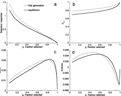
Figure 1 shows the rate of advance, additive genetic variance, normalized skew ( ys = E [ ( G - Z)']/

v",/'),

and kurtosis ( y4 = E[ ( G - 2)4]/

VG

- 3) of breeding values as a function of the mean fitness (i.e., the proportion selected). To emphasize the relatively small cumulative effects of selection on the higher-order cumulants, the additive variance is adjusted so that the heritability is h2 = 0.5 for both the one-generation and equilibrium calculations. In these figures, the truncation point was calculated using the standard formula from Gaussian theory rather than the more elaborate Cornish-Fisher approximation used by ZENC (1987). The differences in the truncation points obtained for these small values of skew and kurtosis are negligible. Following ZENG (1987), the equilibrium moments were calculated using a fourth-order Gram-Charlier expansion. Table 2 shows that higher cumulants rapidly decline to zero, and that adding extra terms to the expansion makes very little difference. (Note that the Gram-Charlier expansion gives a distribution that becomes negative for large

y

if it is defined with an odd number of terms, and may do so with an even number. However, this pathology arises only for y well outside the range of interest.)

The dotted curves in Figure 1, c and d, show the distortion produced by one generation of selection from a Gaussian distribution, while the solid curves show the distortion after the population has settled to a steady advance. These curves are close to each other, showing that the population rapidly equilibrates. Surprisingly, the greatest steady-state skew is produced with relatively weak selection, e.g., with W = 85% for h2 = 0.5. The

(5)

Polygenic Selection Kept Simple

...

first generation

a

\..*

-equilibrium -equilibrium

0.2 0.4 0.6 0.8 1

p. fraction selected

0.2 0.4 0.6 0.8 1

p. fraction selected

C

I

0 ' ' ' c ' ' ' ~ " ' ~ ' ' ' ~ ' ' '

0 0.2 0.4 0.6 0.8 1

p, fraction selected

'1:

...

0.8 ... ...

0.6

1

>O

0.4 -

0.2 -

0 :

0 0.2 0.4 0.6 0.8 1

p, fraction selected 0.006 r

0.004 -

0.002 - In In .-

r"

0:

Y

-0.002 -

-0.004 -

-0.006 -

FIGURE 1.-Response to truncation selection under the infinitesimal model. Individual panels display: (a) the change in mean per generation, (b) the equilibrium genetic variance ( V G ) , (c) the skew (y3 = E [ ( G -

83]1/v,/'),

and (d) the kurtosis (y4 = E [ ( G -

a4]/

v',

- 3), as a function of the proportion selected. All moments are expressed relative to the genic variance, VG,.m,

that would be reached with no selection. The dotted curves give the values after one generation, starting from a Gaussian wth variance VG,F and the solid curves give the steady-state values. Heritability is h2 = 0.5 for both sets of curves. All results were calculated using a fourth-order Gram-Charlier expansion.

TABLE 2

Effects of increasing the number of terms (imax) in the Gram-Charfier expansion (Equation 3) on the predicted change

imax R Skew Kurtosis Pentosis' Hexosis

steady-state kurtosis is also largest when selection is weak; it changes from its most positive value at 55% selected to its most negative value when 98.5% are se-

lected. However, the skew and kurtosis never become large, and have n o appreciable effect on the response to selection, or on the genetic variance. We will show below that the same small effects can be deduced from a purely genetic, rather than statistical, argument.

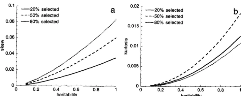
Figure 2 shows how the skew and kurtosis change with the heritability, for

20%,

50% and 80% selection; values are calculated using the fourth-order Gram-Charlier ex-

with the heritability, they never become large. Even when the trait is completely heritable, the skew never rises above 0.1, and the kurtosis never rises above 0.02. Using Fourier transforms: In this method, the distribution after selection is found directly, by multiplying the initial distribution by the relative fitness function. Finding the effect of reproduction directly from Equa- tion 2 would be slow, because it requires two integrations for each value of z. However, the Fourier transform of

(6)

M. Turelli and N. H. Barton

O.' 7 -20% selected

a

0.02 - - -20% selected

:

-

--5O% selected

- -

-50% selected

b,

0.08

-

"--8O% selected .a. - -80% selected /

.

f 0.015 F /

/ /

$

Y

u)

0 0.2 0.4 0.6 0.8 1 0 0.2 0.4 0.6 0.8

heritability

1

heritability

FIGURE 2.-The skew (a) and kurtosis (b) produced under steady truncation selection, as a function of the heritability. Values are calculated as for Figure 1, with proportions selected being 20%, 50% and 80%.

transform (ie., the convolution Equation 2 ) is then given by a simple multiplication, so that

where

Taking the inverse Fourier transform completes the cal- culation,

**(z) =

[

***@)

exp( -

izi)

fi

dx ( 6 4

Numerical results can readily be found by defining the distribution

1Ir(

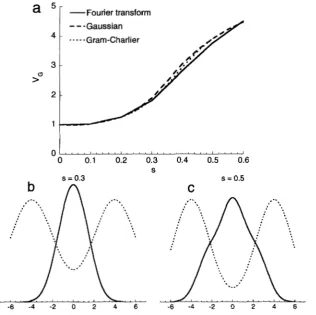
z) on an evenly spaced set of points over some finite range, and then applying the fast Fourier transform algorithm (PRESS et al. 1989). Unfortunately, this does not give a practical way of calculating the slight deviations from normality caused by truncation selection. The discrete approximation causes slight errors in the tails of the distribution, which though small, cause large errors in the variance and higher moments. For example, suppose that the distribution is initially Gaussian, with mean zero and unit variance. Iterating the algorithm over 1 generation with no selection, and with genic variance V , , = 1, should not change the distribution. Table 3 shows that although the error in the distribution itself is small, the variance and kurtosis are inaccurate. Since truncation selection causes only slight perturbations away from normality, the Fourier transform method would require an impracticably fine grid to give sufficient accuracy.

The Fourier transform method is more appropriate for cases in which selection generates large deviations from normality; then, the distribution cannot be adequately described in terms of its first few cumulants. To illustrate this, consider an equilibrium under disruptive selection. We follow FELSENSTEIN (1979) and assume that

the fitness of an individual with phenotype 2 is the sum of two Gaussians: W( z) = exp[ -s( z

-

8)2/2]

+

expi-s( z

+

8 ) * / 2 ] . With environmental variance V,, fitness as a function of breeding value G is

exp[-fYg-

e)2/2]

+

exp[-s*(g+ e ) 2 / 2 ]

W(g) =

_{d m .}

7

(7)

where s* = s/ (1

+

sV,); this is just a smoothed version of the individual fitness.

For simplicity, we consider only the symmetric equilibria at which the population mean is zero. FEEENSTEIN (1979) showed, using a multivariate normal model with constant fitnesses, that these equilibria are unstable when disruptive selection is strong enough that W*(

g)

is bimodal ( c j BULMER 1980, Ch. 10). However, if the two peaks correspond to two different limiting resources, frequencydependent selection can act to keep the mean at zero. [FELSENSTEIN (1979) showed that the

sym-

metric equilibria were only quadratically unstable; thus, weak frequencydependence may suffice.] Although these equilibria are unstable under our constant fitness model, they can be approximated by iterating the recursions beginning with the population mean at zero.

When selection is weak, W* ( g) has a single peak (corresponding to stabilizing selection) ; one expects an a p proximately Gaussian distribution, with variance slightly lower than the genic variance, VG,,. As selection becomes stronger, W*( g) develops two peaks near ? @, and the variance should be inflated above VG,w When selection is very strong, only individuals near

-+e

will

(7)

TABLE 3

Values produced by the Fourier transform method after one generation without selection, starting from a Gaussian distribution with genetic variance and genic variance equal to 1, using grids of different mesh and different ranges of integration

Variance Kurtosis

h a (-83) ( - 6 6 ) (-4,4) (-8,8) (-6,6) (-4,4) AV\Y,axC

32 1.0266 0.9872 1.0027 1.0465 -0.8538 -0.3866 0.022555

64 0.9805 0.9948 0.9971 -0.7535 -0.1043 -0.0361 0.001053

128 0.9829 0.9953 0.9968 -0.6224 -0.0689 -0.0160 0.000633

256 0.9842 0.9955 0.9968 -0.5684 -0.0608 -0.0148 0.000732

The number of points spaced over the range (-8, 8) used for the fast Fourier transform. The range over which the moments were calculated by numerical integration.

'The maximum deviation of the numerically determined probability density function from the expected Gaussian.

a

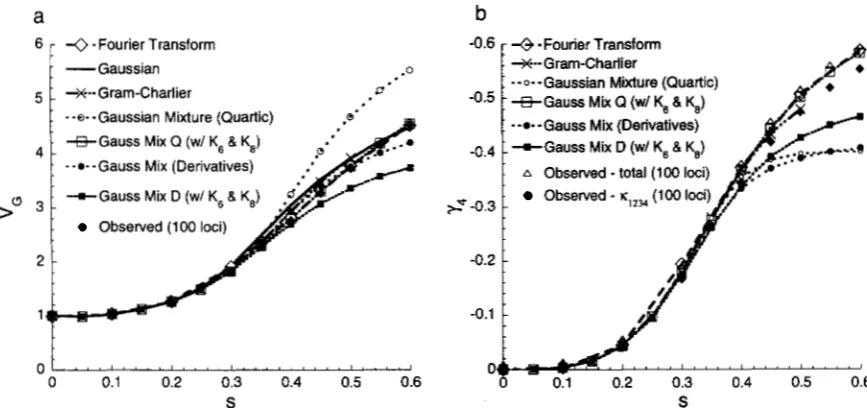
5 - -Fourier transform

-

--Gaussian ---Gram-Charlier

3 - FIGURE 3.-Consequences of disruptive se-

lection under the infinitesimal model. Graph a shows the genetic variance maintained. The solid curve gives values calculated using Fou- rier transforms. The algorithm was iterated for 10 generations, starting from a Gaussian with variance V , = V,. The variance changed little after the first 5 generations, so the generation 10 values are assumed to be near equilibrium. The dashed curve assumes a Gaussian distri-

0 0.1 0.2 0.3 0.4 0.5 0.6 bution and the dotted curve assumes a fourth-

>"

2 -

1

0 " ~ ~ ~ " " ' ~ ~ " ' ~ ~ ~ ~ ~ ~ ~ ~ ~ ' ~ ~ ' ~ '

S order Gram-Charlier expansion. Graphs band

s = 0.3

C

s = 0.5 c show the distribution for s = 0.3 and s = 0.5, calculated using Fourier transforms (solid

curves), together with the graph of fitness as a fimction of breeding value (dashed curves). The fitness of individuals with phenotype xis W( x) =

exp(-s(x- 8)*/2) +exp(-s(x+ O)2/2),where

8 = 4; the environmental variance is V, = 1, and the genic variance is V& = 1.

-6 -4 -2 0 2 4 6 -6 -4 -2 0 2 4 6

Gaussian to a distinctly non-Gaussian distribution; for 0 = 4 and = V, = 1, the transition occurs around s =

0.4.

However, even though the distribution is far from Gaussian, the variance predicted assuming a Gaus- sian distribution [cJ BULMER (1980, Ch. 9)] is close to that calculated using the Fourier transform (dashed us. solid line in Figure 3a). Surprisingly, the Gram-Charlier method does not much improve the fit: adding a fourth- order term makes little difference (dotted line in Figure 3a). Higher order Gram-Charlier calculations are intrac- table. Thus, even when selection maintains a substantially non-Gaussian distribution, the Gaussian approximation for the variance is quite good, and including further cumulants does not much improve it. An alternative, populationgenetic analysis of disruptive selection is presented below.

(8)

GENETIC ANALYSIS

A full description of the dynamics of the allele frequencies and linkage disequilibria that determine the distribution of the trait is more complicated than these statistical analyses. Our approach is based on WRIGHT'S (1935) formula, in which the change in gamete frequencies caused by selection is exactly proportional to the gradient of log mean fitnesswith respect to those gamete frequencies. BARTON and TURELLI (1987) showed how Wright's equation could be rewritten in terms of any other description of the population-for example, the mean and central moments of the genotypic distribution. Since this rotation of coordinates is in general nonlinear, it is accurate only to first order in selection.

TURELLI and BARTON (1990) used this method to approximate the joint effects of weak selection with recombination, and BARTON and TURELLI (1991, Equa- tion

22)

showed how the exact equations under strong selection can be derived from the first-order expressions valid for weak selection. The latter paper described selection by representing the individual relative fitness ( W / w as a polynomial. Here, however, we describe selection in terms of gradients in mean fitness.

Describing the population in terms of cumulants

Our treatment below differs from our previous analyses mainly in that we describe the population in terms of multilocus cumulants, K, rather than the mean m and the central moments C. This approach was applied by BURGER (1991), in his analysis of weak selection on a continuum-of-alleles; he also introduced the use of a generating function to calculate the selection equations. We extend BURGER'S results first by allowing for

strong selection of arbitrary form, and second by allowing for linkage disequilibria among an arbitrary number of loci.

The cumulants are a set of parameters that describe the shape of a probability distribution. The first three equal the mean, the variance, and the third central moment, while the higher cumulants are polynomial functions of the moments. All cumulants have the convenient additivity properties of the mean and the variance (see Equation 12 below). This is particularly useful in analyzing additive polygenic traits: for example, the gradients of log mean fitness with respect to the cumulants of effects at individual loci are the same as the gradients with respect to the cumulants of the overall trait disui- bution. Expressions for the response of the cumulants to selection also simplify the equations for arbitrary multilocus selection. Afurther advantage is that for a normal distribution, the third and higher-order cumulants are all zero. We therefore expect that if the trait is normally distributed, its response to selection can be explained solely in terms of the selection gradients with respect to the mean and variance.

Cumulants bring two disadvantages. First, while the first-order expressions for the response of the non-

central moments to selection are exact and apply for arbitrary selection strength, those for the cumulants are not. Second, the effects of recombination are most natu- rally described in terms of the moments (TURELLI and

BARTON 1990). However, it is easy to move between these alternative representations. We therefore use cumulants to describe selection, but follow changes of the moments under selection and recombination, then convert these to changes in the cumulants.

For a single random variable X , the relations between the cumulants,

Ki,

and the first few moments,

m = E [ X J and C, = E [ ( X - m ) ' ] , are

K, = m, @a)

ti;

= C2, (8b)

1"5

= C37 (8c)

and

I(4

= C, - 3c;. (8d)

The general definition is best given in terms of the moment generating function. Let CT = E( X % ) denote the ith non-central moment. For probability density

f ( x ) , the moment generating function is

f ( 4

=

I-1

exp(xi)j(x) dx, (9a)

and

(The moment generating function is equivalent to the Fourier transform:

f (

2)

=

f(-

i 2 ) f i . ) The cumulants are given by the derivatives of the cumulant generating function, K( 2 ) , which is just the natural log of the moment generating function, i.e.

K(2) = lnV(i)] (loa)

and

The multivariate cumulants are defined in the same way (STUART and Om 1987, Ch. 3) . Now, X is a random vector with probability density

f

(x). The moment generating function is

f ( 2 ) = J-:exp(x.i)f(x) dx

(114

with x ir =

x

x,

ii,

1

and

where C: = E(Xu) and X, = Xi.

Here,

a

u ' f / d f , denotes the partial differential with

(9)

respect to the variables ii in the set U (see Table 1) ; and

C t denotes the expectation ( E ) with respect to f(x) across a set of indices. For example, C t n

=

C:jk = E ( g $ X k ) = a4j(0)/ax@+Jxk. As before, the multivariate cumulants are given by the derivatives of the cumulant generating function, K ( % ) , with

~ ( 2 ) = ln[f(%)]

(124

and

As

noted above, cumulants have a convenient additivity property. Suppose that Z =

z,

Xi,

where ( X l , X,, X,,

.

.) has multivariate cumulants denoted K ~etc. ~ ,

Then Kj, thejth cumulant of the sum Z, is simply related to the multivariate cumulants by

5

=

x

Ku, (12c)

U : I UI = j

where I UI denotes the number of elements in the set U For instance, if 2 = X,

+

X,,

1y2

= K~~

+

K ~ ,

+

2 ~ , ,

(since K~~ = K , ~ ) . Equation 12c follows from the fact that the uni-

variate moment generating hnctionL(2) for Zisjust&(i,

2,

.

, , i ) , where denotes the multivariate moment generating hnction for X. However, we stress that our general treatment does not assume additivity of genetic effects.

We will be concerned with the distribution of docus diploid genotypes,f(x, x*). Here, x is a vector labeling the alleles derived from the mother, and x* the corresponding vector for alleles from the father. With random mating, x and x* are independent in zygotes; but, selection usually generates deviations from multilocus Hardy-Weinberg proportions, necessitating analysis of the joint distribution f(x, x*). However, for compactness, we will set out the methods in terms of a single vector x, which we take to include the states of the full diploid genotype. The expansion to diploid notation is trivial, as indicated in the final equations below (see 19).

The multilocus cumulants defined by Equations 11 and

12 are a new measure of deviation from linkage equilib rium. When more than three loci are involved, they are distinct from those based on the cross-locus moments defined by SLATKIN (1972, Equation 6) and used in our previous papers. They are also distinct from BENNETT’S (1954) principal components, which were defined so as to decline geometrically in the absence of selection. Though cumulants are more convenient for analyzing selection, they are less so for recombination. To see this, consider K $ the

four-locus cumulant after recombination alone. (In terms of central moments, denoted

c,

(12)

implies that KYkl =

GIN

- GjCu - C-,C,, -

C,,qk,

where Cy denotes the covari- ance of allelic effects between loci i and j.) For simplicity, we assume that selection has generated no associations between paternally and maternally derived loci, so that

G,”

= 0 if Uand Vare nonempty sets.

As

in BARTON and TURELLI (1991), we define rs,T for nonoverlapping sets of indices Sand T as the probability of recombination events

that bring together paternally derived alleles from the loci in S with maternally derived alleles from the loci in similarly, rN+ is the frequency of gametes that are “non-recom- binant”with respect to all loci in

N

By converting to central moments, it is easy to show that

~ * e u = T Y M ~ K ~ ~ + (qje0 + qj,u

-

~ J , ~ ~ U D ) K ~ K M

+ (TIkl,klQ + ‘ t j l - r&0510)KikKjl (13)

+ (qjkl,0 + %jk - ql,O~k,@)KdKj~‘

Here, T ~ , ~ 1 - qI, where qY is the recombination rate between loci

i

and j . The factor (

+

qj,

kl

-

rg:pirU 0 ) is

a measure of association between the pair of loci { i j ] and the pair {kl}; it is zero if the event that { i j ] stay together is independent of the event that (kl} stay together. That will be true if the pairs do not overlap on the Same chromo- some (e.&, if they are in the order (i, j, k,

I)

but not ( i, k, j,

I)

)

.

Only if all the loci are unlinked will the cumulant measures of disequilibrium be identical with those of BENNETT (1954).

Response to strong selection: The exact change in genotype frequencies caused by selection is

with

G[x;

yl

= f(X)[S(X -

Y)

-

fW1,

(14b) where S(x -

y)

is the Dirac delta function and W = f ( x ) W(x) dx (see Equations 2.2 and 2.3 of TIJRELLI and

BARTON 1990). With discrete alleles, the integral in (14a) would be replaced by a sum and the Dirac delta in (14b) would be replaced by the Kronecker delta. The crucial step is to describe the population in terms of the moment generating function](%) rather than the genotype frequencies. Using the transformation methods described by Equations 2.4 and 2.5 of TURELLI and BARTON

(1990), we find that, because](%) is a linear function of f ( x ) (see Equation 9 ) ,

with

(10)

Turelli and N. H.

Because recombination produces a linear mixture of probability densities, its effects are simplest to describe for statistics that depend linearly on the density. Thus,

we will describe the effects of selection and recombination on moments rather than cumulants. However, because of the additivity property (1 2), it is simpler to work with selection gradients defined in terms of the cumulants, rather than the moments (see Appendix 1 of TURELLI and BARTON 1990). To achieve this, we replace

The resulting expression for the moments is exact, but is somewhat less elegant than the analogous (first order) equation for cumulants (Bl)

,

since it involves an asymmet- ric ma& @. In terms of generating functions, we have

a

In(W)/af(j;> in (154 by

[a

ln(iir)/aK(j;)l[aK(9)/a~(j;)l.

with

= exp[K(f

+

j;)

-

K@)]

-

exp[K(k)]. As explained below, the matrix G* that gives the response of particular non-central moments C$ to selection gradients on particular multilocus cumulants, denoted K~ can be found by differentiating the generating

function

**6*[x**

91

to produce

A , c % =

E@[Q

VI

(1

7 4

V

where

Here, A, C?, is obtained from A j ( f ) by simply diEeren- tiating with respect to f, ( i . e . , with respect to xi for all loci i E U ) and evaluating the result at f = 0. It is less obvious that the effect of selection on particular cumulants, 2&, is obtained by differentiating with respect to

Pv

This can be verified by working backward from (17a) :

The sum over all V gives a Taylor series in w , hence, (18b) can be written as

From (1 l b ) , we see that (18c) reproduces (16a), and so

verifies Equation

17.

The expressions for G* become complicated for the higher cumulants; for example, G* [ ( z , j , k,

4;

{m, n, o,

p } ]

involves 339 terms. However, Equations 16 and 17 give a compact algorithm that can readily be automated, using a symbolic language such as Muthemuticu

(WOLFRAM 1991). (A description of the routines used to perform these calculations as well as Muthemuticu

notebooks for the Macintosh that implement them are available upon request.) The expression for changes in the cross-locus moments is essentially the same. It is o b

tained by replacing f by (f, f*) and j ; by (j;,

y ) ,

which produces

ACC$,,

=

C@[U,

V

S,

71

2s,,r

d In(

W)

where = ___

a K , 7 '

and

Equation 19 gives the response of the moments to selection on the cumulants. BURGER (1991, Equations 4.4b and 4.6) gives closely related expressions for the change in cumulants, which are also derived from a generating function. His results differ in that they are expressed in terms of the coefficients of a Taylor series expansion of the fitness as a function of breeding value

(his Equation 3 . 5 ) , rather than selection gradients. His results also neglect linkage disequilibrium, and s o are the sum of a set of single-locus analyses. Our equations are essentially an extension of his analysis to arbitrary multilocus systems and to strong selection.

Allowing for recombination: The exact effects of strong selection on the non-central moments are given by Equation 19. This equation makes no assumptions about the mapping of genotypes onto phenotypes. It requires only that the distribution of genotypes can be specified in terms of moments. As discussed in BARTON and TURELLI (1991), this is straightforward for diallelic loci or models with additive allelic effects. Recombina- tion is then dealt with using Equations 14 and 15 of

(11)

describe deviations from normality, and they simplify the characterization of the distributions of breeding values and phenotypes under the additive model.

Calculating the selection gradients under an additive model: We will now restrict attention to a simple additive model for polygenic inheritance. Letting Z denote the phenotype of a randomly chosen individual, we assume

n

Z = ( X ,

+

X:)

+

8 G + 8,

(20)

I= 1

where Xi(Xy) denotes the additive contribution of the maternally (paternally) inherited allele at autosomal locus

i,

G denotes the total genetic contribution, and

8

denotes a random, Gaussian-distributed environmental effect with mean 0 and variance V,, which is independent of G. Under this model, I$, the jth cumulant of the distribution of phenotypes, is the sum of the jth order cumulants across all sets ofjloci (plus

V, for the second cumulant) (see Equation 12). Hence, the selection gradient with respect to any cumulant involving j loci is the same as the selection gradient with respect to the jth cumulant of the genotypic (or phenotypic) distribution. In particular, the terms

2esT

in Equation 19a reduce to

Y j

=

a

In( I%‘)/aK, with j = I S

+

TI, the total number of indices in the sets Sand T. (This reduction occurs with any distribution of environmental deviations, %, as long as

8

is independent of G.) We now describe how these genotypic gradients can be calculated.

We first find how the distribution of phenotypes, f (x),

depends on K,. The Fourier transform of a distribution,

f

(Equation 6b), is equivalent to its moment generating function,

f

(Equation 8a), which in turn can be written as a Taylor series in the cumulants (Equation 9), i e . ,

Hence,

Taking the inverse Fourier transform (Equation 6c) of Equation

22,

This simple relation can now be used to find the selection gradient,

W j ! dxJ dx.

This can be interpreted in two ways. First, consider how the mean fitness changes when the distribution is translated by T, so that f ( x ) becomes f ( x - r ) , and af/ax = -af/ar. Setting

we have

Thus, the selection gradient with respect to the jth cumulant is proportional to the jth differential of the log mean fitness with respect to translation of the distribution. Another relation can be found by integrating Equa- tion 24 by parts j times:

Thus, the selection gradient

Zei

is also proportional to the expectation of the jth differential of the relative fitness. Note that (25b) and (26) are generalizations of the formulas provided by LANDE (1976) and LANDE and

ARNOLD (1983) for the “directional selection gradient,”

p

=

a

In( F;i3/aZ, calculated under the assumption that the distribution of phenotypes remains precisely Gaus- sian (so that 7 is just

2).

In this case,

2,

=

p.

Similarly, i f f ( x ) is Gaussian, Equation 26 implies that

Z2

= y/2, where y is the univariate version of the “stabilizing selection gradient” defined by LANDE and ARNOLD (1983, Equation 14b; c$ MITCHELL-OLDS and SHAW 1987).

Approximating the selection gradients: Calculations for specific models are simplified if one can characterize the distribution of breeding values (at least approximately) in terms of a finite set of cumulants. This can always be done for a finite number of loci and alleles. For example, with biallelic loci, the distribution ofgenotypes

is completely characterized by cross-locus cumulants involving distinct loci ( K ~etc.) and the allele frequencies ~ ~ ,

(12)

parameters, one can also approximate the

Ti

“para- metrically” by first differentiating the density with respect to the cumulant then integrating. This will not generally give the same result as Equation 26, because as the lower cumulants vary, the higher cumulants change with them, in a way that depends on the class of distributions considered. For small departures from normal-

ity, we will show that the Tj can be well approximated from Equation 26 assuming that f (x) is Gaussian.

Another approach is to derive the selection gradients from a polynomial approximation to the fitness function. This is the method used by BARTON and TURELLI

(1991); there was a slight error in the relation between the polynomial coefficients and the gradients given in AppendixA of that article, which is corrected in APPENDIX

A below. This polynomial approximation is also related to BURGER’S (1991) Taylor series expansion of fitness. If the genotypic (or phenotypic) fitness function is a polynomial, we can directly express the mean fitness as a function of the cumulants of the distribution, then dif- ferentiate to obtain the Tt. For instance, if the genotypic fitness function is the quartic,

W(x) = 1

+

b l x + b,?

+

b 3 2

+

b4x4,

(27)

then

W =

W(Z)

+

VJb,

+

3b3Z-t 6b4-P)

(28)

+

K3(b3

+

4b‘Z)

+

b4(K4

+

3v-3

=

+

V,(3b3

+

12b4Z)

+

4b4K3, (29a)

WT3 = b3

+

4b4Z,

and

m4

=b4

Note that if we were working with central moments rather than cumulants, the partial derivative of In( W ) with respect to the second moment would differ from (29b) because the coefficient of b4 in

(28)

would be simply C, =

E [ ( 2 -

a‘],

and hence would not contribute.

If W( x) is not a polynomial, it will generally not be possible to calculate the

Ti

exactly without assuming a distribution of breeding values. However, many selection regimes, including truncation selection, can be adequately approximated by a quartic over a range of genotypes that includes most of the population; so that

Ti

for

i = 1-4 often suffke for approximating the dynamics. According to the Gaussian infinitesimal model, %l and

9,

suffice. We will use a fourth-order description to approximate the multilocus effects of truncation selection. We will show that under truncation selection, and pre- sumably most forms of directional and stabilizing selection, the cumulative effects of third- and higher-order disequilibria are negligible. This is not true, however, for

strong disruptive selection.

Several criteria are possible for approximating an arbitrary fitness scheme by a polynomial, such as mini- mizing the “distance” between the exact and approximate fitness functions. To predict selection response, however, it seems more natural to approximate the distortion of the distribution of breeding values or phenotypes. This is most easily accomplished by considering how selection alters the non-central moments. LetCT denote the ith non-central moment before selection, and let C.* denote its value after selection. If the fitness function is

n

W(x) = bp’, with bo = 1, (30)

i = O

then

n n

W= x b i C T and

Wc*

= $CT+j. (31)

i=O j = 0

Hence if we know how a selection regime changes the noncentral moments, we can use (31) to find a polynomial of order n that produces the same changes in the first n moments (and cumulants). Let A,CT = CT“

C$ b = ( b l , bz,

. . .

,

b,)T, and A,C* = (A,CT, A,C$,

.

. .

,

A,C;)’, and define the n X n matrix A = ( aii) by aij = CT+j - C F y * (the superscript Tdenotes

transpose). Then the coeffkients of the approximating polynomial are

Under the Gaussian infinitesimal model, changes in the first two moments completely characterize the selection regime, so a quadratic approximation suffices, as noted by LANDE and ARNOLD (1983). For non-Gaussian

distributions, changes in the higher moments are also relevant. These may be estimated empirically. In general, however, one must know the initial distribution of breeding values to predict the effects of a given W( x). Because truncation selection produces only small departures from normality, it suffices (as shown numerically below) to consider how selection alters the distribution assuming that it is initially Gaussian. If only individuals with phenotypes 2

>

t survive, the genotypic fitness function is

(33)

where @(x) is the cumulative normal density and

a,

is the environmental standard deviation. Assuming the current mean of the population is 2 and its phenotypic standard deviation is a, let

p

denote the fraction of the population that survives truncation selection, let t* = ( t - Z ) / a , denote the normalized truncation point, and let

I(

p )

= exp[-(t*)‘/2]/

(13)

I

1 .o

0.8

u) 0.6

E 0.4

I

0.2

0.0

-0.2

0 1 2 3 4 5 6

breeding value

FIGURE 4.-Comparison of the third-order (dashed line) and fourth-order approximations (open symbols) obtained from (32) to the exact truncation fitness function (33) with the fraction selected,

p ,

equal to 0.2 and 0.8 with V , = V, = 1.

1989, Ch. 11). Applying Equation 26 under the assumption that the distribution of breeding values is Gaussian, we obtain

for

i

= 1 , 2 , .

. .

,

where E denotes expectation with respect to a standardized normal density, Hi denotes the ith Hermite polynomial, h = crJa,is the square root of the heritability, and

t^

= -fa,/a,. The first four

Yi

are

and

Z1

and LEz are identical to the "parametric" values obtained by differentiating with respect to the parameters of the Gaussian density. The fitness gradients

(34b) are identical to those obtained from the polynomial approximations (32) under the assumption

h i= K ~ .

2l

+

K ~ . .

2z

+

K,

...

33 +

K,

....

Z4,

A K ~ =

A K ~

-

A K ~ A K ~ ,

- 0 . 5 ~ ~ " ' ~ " ~ ~ " " " " "

0 0.2 0.4 0.6 0.8 1

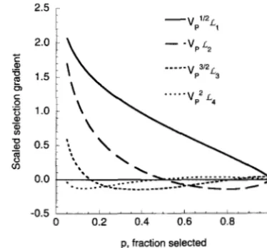
FIGURE 5.-The dimensionless selection gradients, V? for i = 1-4, obtained from (32) and (34) with

p

ranging from 0.05 to 0.99.

that the distribution of breeding values is Gaussian. [In general, if the initial distribution is Gaussian, both (24) and the polynomial scheme (32) lead to the general expressions provided below for the

2i,

see (44) and (48).]

Figure 4 displays the close fit of the fourth-order approximations obtained from (32) to the exact truncation fitness function (33) with

p

= 0.2 and 0.8 and V, = V, = 1. The polynomial approximations are multiplied by a constant to produce the correct The quartic

approximation is very accurate for all breeding values within three standard deviations of the mean, but the cubic approximation is much cruder. The dimensionless selection gradients, V$z3ifor

i

= 1-4, obtainedfkom (32) and (34), are displayed in Figure

5

with p ranging horn 0.05 to 0.99. Note that the third- and fourtha-der gradients are much smaller than the first two.

(14)

926 M. Turelli and N. H. Barton

Here

A

denotes the change in the cumulants that would be observed if selection were so weak that products of the

Zei

could be ignored; and rN= 1 - rNg denotes the frequencywith which recombination disrupts the loci in the set N ( i.e., the fraction of gametes that are not parental haplotypes at these loci). In each equation, we have indicated sums over a particular subscript by

‘‘-”

(e.g., K ~ . . =

xi,,

K ~ J . Equation 39 is abbreviated by using

“. .

.”

to denote the two additional terms in each

sum obtained by permuting the subscripts

i,

j , and k in the first term.

The expression for the fourth-order disequilibrium is more cumbersome. In general,

AK~,,

= A K ~ , , -

[ A K ~ ( A K ~ ~

+

3 h l ~ j k l )

+

3 similar terms] - [ ( A K ~

+

Y ~ K J ( A K , ,

+

r,,~,,)

+

2 similar terms]

(40)

+

~ [ A K ~ A K ~ ( A K ~ ,

+

r , , ~ , , )

+

5 similar terms] -

~ A K ~ A U , A K ~ A K ~ ,

where the “similar terms” are generated by permuting the indices. The general form of A K ~ ~ , is unwieldy, so we will

restrict attention to exchangeable, unlinked loci ( L e . , unlinked loci with equal effects on the character and identical allele frequencies). In this case, for distinct

i,

j , k and 1,

7

A K q k , = - s K +

+

i K q k l . 3 1 1

+

(;K%. f 2Ki.Kqk.

+

;K+..)%z

+

( I ~ K : . K ~ .

+

i K p K q . . f 3Ki..Kq,.

+

3Ki.Kqk..

+

;Kvkl...)%3

(41)

+

(24~:.

+

7 2 ~ ~ .

Ki.. Kq.

+

36~:. Kq..

+

9

5 K i . .

+

4K j... Kqk.

+

6Kq. KY..

+

6Ki.. Kqk..

+

4Ki. Kqk...

+

gKqkl 1

....

)x4.

These recursions were checked by numerical multilocus calculations as described below. If the fitness function is a fourth-order polynomial, they are exact. If the fitness function is more complex, additional terms involving

xi

for

i

2 5 appear. Nevertheless, Equations 35-41 will often provide a very accurate approximation for selection response, as demonstrated below for truncation selection.

Departures from normality at the infinitesimal limik To predict the deviation from normality under strong selection, we add the recursions (35)-(41) across loci to produce recursions for the cumulants of the distribution of breeding values. Under the additive model, departures from normality arise from linkage disequilibrium and from the fact that only a finite number of loci contribute to the trait (BULMER 1980, Ch. 8; BARTON and TURELLI 1989). At linkage equilibrium, the central limit theorem implies that, under suitable restrictions on the relative contributions of individual loci, the distribution of breeding values will become Gaussian as the number of loci approaches infinity. For a finite number of loci, the distribution will not be Gaussian if the distributions of allelic effects at individual loci are non-Gaussian. To disentangle the roles of disequilibria and the distributions of allelic effects, we will first consider the simpler case in which a very large number of loci with comparable effects contribute to the trait. As discussed by TURELLI and BARTON (1990) and derived in greater generality in APPENDIX B, in the infinitesimal limit only terms of the form K~ in which the set U contains k distinct indices contribute to the kth-order cumulant for k 2 3. Using this and assuming unlinked loci, Equations 35,36 and 38 imply the following recursions, complete to T4, for the mean phenotype and the genetic variance:

AVG = $VG,m - VG)

+

$&

+

(v‘,

+

$,)%,

+

(3VGK3

+

$5)%s

+

( 3 g

+

4VGK4

+

$$f4 - (43)

where Ki denotes the ith cumulant of the distribution of breeding values and VG,, denotes the “genic variance” ( 2 x K J which remains constant.

If the distribution of breeding values is Gaussian, K j = 0 for

i

2 3. Applying Equation 24 to the phenotypic fitness function, we see that

A,Z As Vp

+

(AsZ)2

VP 2vp

.

g

= - and g2 = ₍₄₄₎

Thus, (42) reduces to the standard selection response equation, (1); and (43) reduces to BULMER’S (197l)equation

A V G = $h4As Vp

+

5(

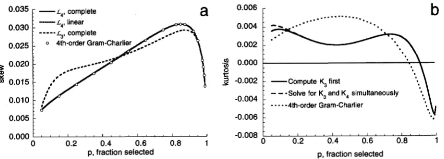
1 V,, - VG). (45)

(15)

0.035 - L ~ , complete

a

0.030

1

0.025

1

2

0.020

!

Y

v, 0.015

0.010 f

-

L ~ , linear

0.005

0.000

0 0.2 0.4 0.6 0.8 1

0.006 -

_b

..--“”“-”

”..

...

0.002 -

.$ 0.000

2

3

-0.002 -

:

-

Compute K, first

-0.004 -

:

-.

- -

-4th-order Gram-Charlier

-0.006 -

- 0 . 0 0 8 ~ ’ ’ ~ 1 . . ” ’ ’ ” . ~ “ . ’ ~ 1

0 0.2 0.4 0.6 0.8 1 p, fraction selected

FIGURE 6.-Consequences of continued truncation selection under the infinitesimal model. Graph (a) presents approximations for the equilibrium skew for various

p

with h2 = 0.5, using (34) for the selection gradients. The “linear” approximation is (49), and it is indistinguishable from the “complete” approximation. Graph (b) presents analogous approximations for kurtosis. See text for details.

then

AK3 = - i K 3

+

i K 4 g l

+

(qVGK3

+

:K5)Z2 i- [iV:

+

!(e

+

VGK4)

+

;K6]T3

( 4 6 )

+

( 9 G K 3

+

y K 3 K ,

+

3VGK5

+

f K , ) 2 , -

$0(2?)

terms from AVJAZ

+

!(AZ)’.

Similarly, we can abbreviate the exact expression, up to

2,,

for AK4 as

A partial consistency check on these recursions is obtained by assuming that the distribution of G is initially Gaussian. In this case, Ki = 0 for i 2 3,

2,

and 5 f 2 are given by ( 4 4 ) ,

AsK3,p

+

3A,VpAsZ

+

(A,Z)’

23

=

6 V : ( 4 8 4

and AsK4,p

+

3(A,Vp)2

+

4A,K3,,A,Z

+

6A,Vp(A,Z)2

+

(A,Z)4

24 V;

g4 =

,

where Kz,p denotes the ith cumulant of the phenotypic distribution. It follows from ( 4 6 ) , ( 4 7 ) and ( 4 8 ) that AK3 =

h6A,K3,p/4 and A K , = haA,K,,p/8, as expected.

Truncation selection: Recursions ( 4 2 ) , ( 4 3 ) , ( 4 6 ) and ( 4 7 ) are generally difficult to apply, because each AKi

depends on higher-order cumulants. Thus, no “closed” system of equations can be obtained without assumptions. The simplest generalization of the Gaussian infinitesimal model is to assume that cumulants of order k 2 3 can be

adequately approximated by ignoring cumulants of still higher order. This is likely to be accurate only if the cumulants form a decreasing sequence. The consistency of this assumption can be checked by applying it successively to each