© 2018 IJSRCSEIT | Volume 3 | Issue 5 | ISSN : 2456-3307
ANN Approach for Error Optimization in Process
Synchronization Using Back-Propagation Algorithm
Sayma Bano, Neelendra BadalDepartment of Computer Science & Engineering, Kamla Nehru Institute of Technology, Sultanpur, Uttar Pradesh, India
ABSTRACT
The work includes in this paper is inspired from the convolution involved for solving the problems by a neural network. The aspiration of this paper is to demonstrate the minimization of error for problem-solving techniques, like process synchronization, Classification etc. The work includes three Artificial Neural Network Algorithms i.e., Feed-forward, Back-propagation and Output-Hidden Weight Optimization. Optimization is being achieved with the minimized error rate for the problem-solving using neural system approach.
Keywords: Back-propagation Error Methodology, Optimization, Synchronization
I.
INTRODUCTION
The paper considers two different cases of the neural net architecture. It describes the error reduction in the problem-solving techniques by means of neural net algorithms. To minimize such error rate three methodologies like feed-forward, back-propagation and Output Weight Optimization-Hidden Weight Optimization are being revealed in this paper. The paper initiates an illustrative note on the artificial neural system. It also demonstrates the error optimization and synchronization by using back-propagation methodology. At last the tentative work is being disclosed in this paper.
II.
REVIEW OF PREVIOUS WORK
This section offers the review of the related previous work. The first structure of neural net was proposed by McCulloch and Pitts in [9]. This structure contains one neuron at the output-seam and two neurons at the input-seam. Richards in [12] demonstrated the neural system into three layers i.e. input-layer, hidden-layer, and an output-layer. Later
on; the weight cost of the neurons was updated by Rosenblatt in his research work in [13]. Nguyen and Hoff in [10] developed a mathematical formula for minimization of error in the neural network. The innovative idea of Back-propagation algorithm was invented by Werbos Parker et al. in their paper [18]. The Back-propagation learning algorithm in multi-layer perceptron networks was introduced by Atkinson and Tatnall in [3]. OWO-HWO was proposed in [4], [15] by …. To solve the linear equations for the weight in output-layer and reduces the training error rate. Jain et al. in [7] developed various types of paradigms related to the learning rules, architecture and algorithms. Hopfield in his paper [5] applied a particular nonlinear dynamic structure for solving the problems in optimization.
III. METHODOLOGY
i.e. Feed-forward, Back-propagation and Output-Hidden Weight Optimization [4], [15].
A. Artificial Neural Network
Nicolette [11] defines the ANN as a computational network consisting of many parallel neurons that communicate with each other through weighted interconnections in order to perform the particular task. The intensity of the problem-solving network depends on the number of neurons their interconnection and how each neuron work [1].
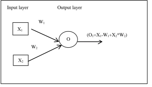
The figure1 shows a simple ANN structure. It contains two layered structure such as the input layer and the output layer. The input layer contains two neurons (nodes) i.e. X1 and X2. The output layer
contains only one node i.e. O. Each layer neurons is connected to its next higher level neurons through a weighted (biased) connection. ANN restricts the connection of the neurons of the same layer. The input layer propagates the entire data signals to the output layer via hidden layer.
Figure 1. Simple ANN Structure
The figure1 of ANN shows that the output layer node of the problem-solving network has two dependencies i.e. X1 and X2. The out value of the
output layer neuron is calculated by taking the summation of the weighted connection multiplied by the given input signals [16]. This formula is used for each layer neurons including the hidden layer neurons.
B. Ann Architecture
The artificial neural network architecture entails groups of innumerable neurons that are arranged in a layered structure. The figure 2 shows the layered structure of problem-solving neural network. In this structure the lowest layer i.e. layer 0, is called the input layer, the next higher layer i.e. layer 1, is called the hidden (unseen) layer and the final layer i.e. layer 2, is called the output layer [12]. In the input layer, each neuron assigns input signals from an outward source. All the computations or processing is made at the hidden layer and its computation is completely unseen to other layers. It also transfers the result to the final layer and then to the outer system. Each layered neurons join with the other layered neurons through a weighted cost connection. The every neurons of the network is always connected to its adjacent layer neurons by an interconnection. It is noted that no neurons of the similar level in the problem-solving network can link with other neuron of the layer.
Figure 2. A Multi-Layer Network
IV. ANN ALGORITHMS
An ANN Algorithm involves bit by bit procedure for minimizing the error. It renovates the weight cost of individual neuron at every single layer. The neural network algorithm includes are Feed-forward, Back-propagation [18] and Output-Hidden Weight X1
Input layer Output layer
X2
O W1
W2
(O1=X1*W1+X2*W2)
I1
I2
L1
L2
O1
Input layer (I) Hidden layer (L) Output layer (O)
Output W (I1, L1)
W (I2, L2)
W (I2, L1)
W (I1, L2)
W (L1, O1)
this paper are demonstrated with the help of flowchart diagram in Figure 3.1.
The primary phase entails setting the initial value to separate neuron of the initial layer. These values are selected from an outside source.
The subsequent stage allocates the weight rate to each interconnected nodes of the problem-solving network grid.
The third step calculates the production rate for individually layered neurons by using a feed-forward algorithm.
The next step encompasses the fixed target value for the calculation of error rate in the neural system. The calculated value obtained is matched with the given target value. If the obtained value is not matched by the
wanted target value, then consider the backpropagation algorithm.
The last step includes updating each weight of connected neurons at the output-Hidden tier of the system. And it also involves estimating the error cost for each layered nodes in the network.
Figure 3.1. Flowchart of Algorithm
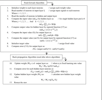
A. Feed-Forward Algorithm
The feed-forward algorithm [8] involves a transfer of signal from the primary layer to the unseen layer and then reaching to the resultant (final) seam. Each neuron of every level is linked to its succeeding level neurons by a biased cost link. The weighted connection should be a small random number which lies from -1 to +1. The given input value is accelerated in an onward path from the lowest layer to unseen level and then passes to the last resultant level through a weighted cost interconnection. The hidden layer performs the whole calculation for finding the best results for the production (final) layer. The resultant value of an individual neuron is calculated by taking the summation of the given input signal multiplied by the weighted cost link that depends on those prior neurons. The target rate is fixed for calculation of the error value in the neural network system. The first error calculated at output level is done by a feed-forward algorithm. The algorithm stages are revealed in figure 3.2.
B. Back-Propagation Algorithm
The back-propagation algorithm [3, 14] is established for solving the reduced error rate in the problem-solving system. It is used when the calculated value acquired from the problem-solving net is not matched with the given target value, then it back-propagate to its previous layer this method is called propagation and the procedure is called back-propagation algorithm. The algorithm involves a repetitive method in the problem-solving network. It updates the weight [6] of each layered neurons i.e. output-hidden layered neurons and also find the error for separate level neuron. The procedure is continued till the acquired value is matched with the given target value.
Initialize the input signal to an input layer
Initialize the weight to each layer node
Apply feed-forward algorithm
Compute the output value for each layer node
Initialize target value
Calculate error at the output layer
Match Stop
Yes Apply
Back-propagation algorithm Update hidden layer
weight Calculate hidden
layer error Update hidden
layer weight
C. Output Weight Optimization-Hidden Weight Optimization (O-H Weight Optimization) O-H is another approach another for adjusting the weights cost of output-hidden layer. The methodology is used in forwarding direction for optimization of weight at the output-hidden layer. It
decreases the error rate of hidden-layer by using the
hidden-layer weights. The O-H Weight
Optimization follows the algorithm the steps from 10 to 12 as revealed in figure 3.2.
Figure 3.2. ANN algorithms
V.
RESULTS AND ANALYSIS
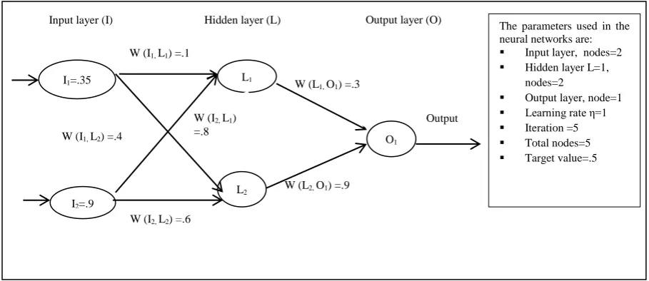
The work involves considering two different cases of the neural network architectures that show minimization in error. Considering, the first neural network structure, the network comprises three-layer i.e. the primary three-layer is the input three-layer, it contains two nodes. Secondly, is the hidden layer, It
has one node. The network contains total five nodes i.e. it acquires two nodes at the initial layer, two nodes at the unseen layer, and one node at the final layer. Each layer nodes is attached with its following layer node through a biased value link and no connection should be there among the nodes at the same layer, as exposed in (fig: 4a).
Feed-forward Algorithm
1. Initialize weight to each layer neurons // assign each weight value
2. Read number of neurons in input layer Ii // assign input signals to each neurons
Where i = 1, 2, 3 …
3. Read the number of neurons in hidden and output layer
4. Compute the input value (inLjk) for hidden layer as: // for single hidden layer put k=0
Where j = 1, 2, 3….. And k = 1, 2, 3…..
inLjk= 𝑛𝑖=1Ii ∗ Wijk
5. Compute output value for hidden layer by sigmoid function [17] as: outLjk= (1/(1+e(-inLjk)))
6. Compute the input value (Oi) for output layer as:
inOi = 𝑛𝑖=1outLjk ∗ Wjk
7. Compute the output value (out Oi) for output layer by sigmoid function [17] as:
outOi = (1/(1+e(-inOi)))
8. Initialize target value // assign fixed value
9. Compute error (∂ Oi) for output layer as:
∂Oi= (target-outOi)*(1- outOi)*(outOi)
Back-propagation Algorithm (used after above algorithm)
10. Update weight (Wjk+) of output layer as: // where η is fixed learning rate value
Wjk+=Wjk+η(∂Oi*outLjk)
11. Compute error for each hidden layer neurons as:
∂Ljk= (outLjk)(1- outLjk)( 𝑛𝑖=1(∂Oi ∗ Wjk+))
12. Update hidden layer weight (Wij) as: // calculate new hidden layer weight
value
Wij+=Wij+η(∂Ljk*Ii)
Figure 4a. A neural network with one node at the output layer
The neural network system has static learning rate value and a permanent target value. The problem-solving network uses the three methodologies i.e. Feed-forward, Back-propagation, and O-H Weight Optimization algorithms. In feed-forward [8] the primary signal propagates in a frontward track and it analyses the output (production) value for each layered node and then computes the first error rate at the final layer of the neural system. If the final value calculated is not matched with the wanted target value then it propagates back to its earlier seams, this procedure is called Back-propagation and the course is called propagation algorithm. In back-propagation algorithm, it first adjusts the weight cost of the output layer. After that it determines the error
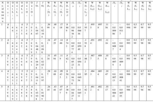
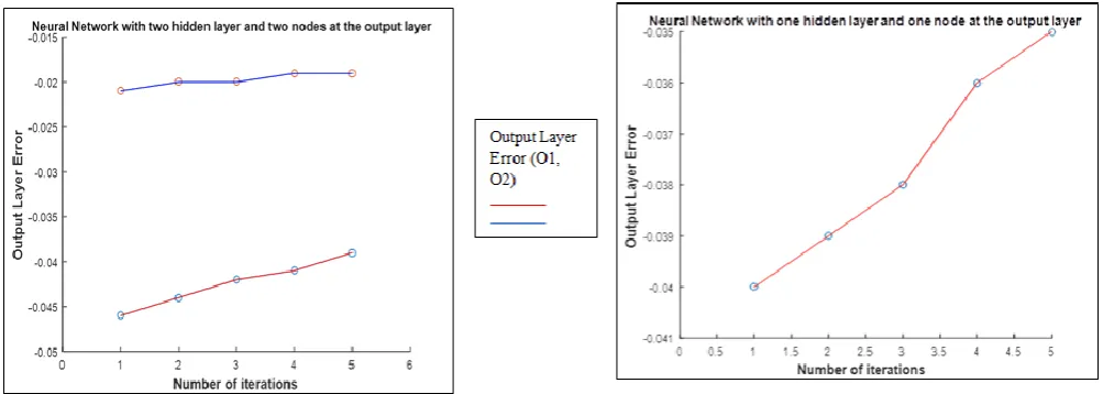
value for individual node of the hidden-layer in the system. The algorithm determines the error value of the hidden-layer for the problem-solving network. It adjusts the weight cost of the unseen-level for the problem-solving network. This procedure is continued till the obtained value is matched or closest to the desired target value; all the calculation is done only up to five iterations. All the estimated charges are disclosed in the table: 4a and the graph plotted in figure 4c display the minimization of error per iteration.
The Formula used for the calculation at the output layer
Error = output value*(1-output value)*(target-output value) ……….. (1)
New Weight = previous weight value + learning rate value*(Error of next node*output value of the previous node)...….…. (2)
The Formula used for the calculation done at hidden layer
Error = output value*(1-output value)*(summation (Error of next node *weight from previous to next node))………….. (3)
New Weight = previous weight value + learning rate value*(Error of next*input value) ………….. (4) I1=.35
I2=.9
L1
L2
O1
Input layer (I) Hidden layer (L) Output layer (O)
Output W (I1, L1) =.1
W (I2, L2) =.6
W (I2, L1)
=.8 W (I1, L2) =.4
W (L1, O1) =.3
W (L2, O1) =.9
The parameters used in the neural networks are: Input layer, nodes=2 Hidden layer L=1,
nodes=2
Output layer, node=1 Learning rate η=1 Iteration =5
Total nodes=5
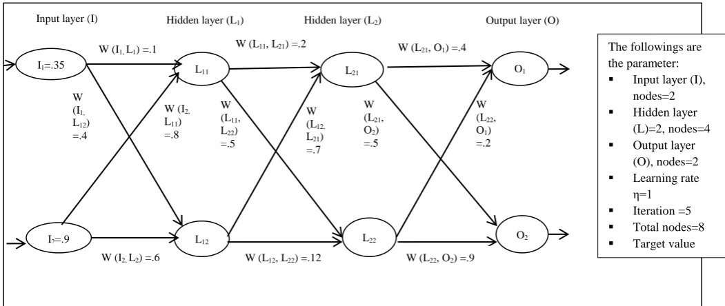
Table 1. contains the calculated rate of the neural net containing one node at the output-layer: architecture. The net comprises of one initial input-layer, 2 hidden layers, and one production level. The network contains total 8 nodes i.e. it contains two nodes at the lowest input layer, two nodes at the primary hidden-layer, two nodes at the secondary hidden-level, and two nodes at the final layer, as presented in figure 4b. The problem-solving net has stable learning rate. On expanding the node range at
the output-layer, the system reveals different variation in the graph plotted in figure 4c.
It also uses the same algorithms for the estimation of error cost and renovating of weights cost of the neural system. All results are determined and exposed in the table: 4b and the graph mapped in figure4c indicate the minimization of error per iteration.
Figure 4b. A neural network with two nodes at the output layer I1=.35
The followings are the parameter: Input layer (I), Learning rate
η=1 Iteration =5 Total nodes=8 Target value
The figure 4b network uses three algorithms i.e. feed-forward, back-propagation, and O-H weight optimization [4], [8], and [15]. All the result is obtained by using the same formula as it is done in the preceding case of the neural net architecture. In feed-forward it analyses the output-value for separate neuron at every layer and at last, it determines the error charge at the output-layer by using equation (1). The fixed target value is assigned to each individual node of the final-seam. The value determined is not matched with the static target value, then reverse back to its last layer using a back-propagation
algorithm. In back-propagation, output-layer weight cost is changed by using equation1, & 2. It also analyses the error rate for every neuron at hidden layer by using equation 3.
The optimization algorithm involves updating of the weight-cost at each layered neurons including output-hidden layer. The parameter for the net is revealed in figure 4b. Each weighted connection assigns a random number. And the input value allocated to the input-layer is also chosen randomly.
Table 4b. includes the estimated value of neural grid with two nodes at the output- layer: N 0.1585 (For Neural-Network with 1-hidden layer and one node at the output-layer) Old Error ∂O1 = 0.1936, New Error ∂O1 =
-0.1598 and Old Error ∂O2 = -0.1038, New
Figure 4c. Both Graph shows the minimization of error at the output layer
VI. CONCLUSION AND FUTURE SCOPE
From above discussion, the conclusion is drawn to attain the reasonable results in reducing the error rate in the neural net by means of the feed-forward, backpropagation and O-H Weight Optimization algorithm. The first error rate is analyzed at the output-layer by a feed-forward algorithm and if the value obtained is not matched with desired value then, the backpropagation algorithm is used. The back-propagation algorithm updates the weight for separate seam and computes the error value for every layered neuron. All the calculation is disclosed in the table 4a & 4b for up to 5-iteration and graph drawn in figure 4c display the minimization in error rate in the neural net. The work is implemented with the consideration of one hidden-seam and two hidden- layers. Further, it may be extended for a number of layers for more than two-layers and may be identified for the difficulty involved for numerous layers.
VII.
REFERENCES
[1]. I., Abu-Mahfouz, "An Absolute Study of Three Artificial Neural Networks for the Detection and Classification", In International Journal of General Systems, vol.34 (3), pp. 261-77, 2005.
[2]. M.,Alsmadi, K., Omar, and S., Noah, "Back-Propagation Algorithm: The Best Algorithm among the Multi-layer Perceptron Algorithm", in International Journal of Computer Science and Network Security, vol.9 (4), pp.378-83, 2009.
[3]. P., Atkinson, and A., Tatnall, "Introduction Neural Networks in Remote Sensing", In International Journal of Remote Sensing, vol.18 (4), pp.699-709, 1997.
[4]. H.H, Chen, M.T, Manry, H., Chandrasekaran, "A Neural Network Algorithm Developing multiple Sets of Linear Equations", Neuro-computing, vol.25 (1-3), pp.55-72, 1999.
[5]. J.J, Hopfield, "Neural Networks and Physical System with emergent collective computational abilities", In Proceedings of National Academy of Sciences of the USA, vol.79 (8), pp.2554-2558, 1982.
[6]. T., Jayalakshmi, and A.,
Santhakumaran,"Improved Gradient Descent Back-Propagation Neural Networks for Diagnoses of Type II Diabetes Mellitus", In Global Journal of Computer Science and Technology, vol.9, pp.94-97, 2010.
[7]. A.K., Jain, J., Mao, and K.M.,
[8]. L.K., Li, S., Shao, and K.F., Yiu,"A New Optimization Algorithm for single Hidden layer Feed-forward Neural Network", applied In Soft Computing, vol.13 (5), pp.2857-62, 2013.
[9]. W.S., McCulloch, and W., Pitts,"A Logical Calculus of ideas immanent in neurons activity", Bulletin of Mathematical Biophysics, vol.5, pp.115-133, 1943.
[10]. D., Nguyen, and B., Windrow, "Improving the Learning Speed of 2-layer Neural Networks by choosing Initial Values of the Adaptive Weights", Proceedings of the IEEE International Joint Conference on Neural Networks, vol.3, pp.21-26, 1990.
[11]. G., Nicolette, "An Analysis of Neural Networks as Simulators and Emulators", Cybernetics and Systems, vol.31 (3), pp.253-82, 2000.
[12]. J., Richards,"Remote Sensing Digital Image Analysis", Berlin: Springer-Verlag, 2006. [13]. F., Rosenblatt, "The Perceptron: a probabilistic
model for information storage and organization in the brain", Psychological Review, vol.65, pp.386-408, 1958.
[14]. D.E., Rumelhart, G.E., Hinton, and R.J., Williams, "Learning Representations by Back-propagating Errors nature", vol.323, pp.533-536, 1986.
[15]. M., Sheikhan, A.A., Sha’bani, "PSO-Optimized Modular Neural Network trained by OWO-HWO Algorithm for Fault Location in Analog Circuits", in Neural Computation Application, vol.23 (2), pp.519-530, 2013.
[16]. T.S., Wang, L., Chen, C.H., Tan, H.C., Yeh, and Y.C., Tsai, "BPN for Land Cover Classification by using Remotely Sensed Data", In Proceedings of Fifth International Conference On Natural Computation, IEEE, pp.535-9, 2009.
[17]. A., Wanto, A.P., Windarto, D., Hartman, and I., Parlina, "Use of Binary Sigmoid Function And Linear Identity In Artificial Neural Networks For Forecasting Population Density",
In International Journal of Information System and Technology, vol.1 (1), pp.43-54, 2017. [18]. P., Werbos, "Generalization of