International Journal of Computer Science and Mobile Computing A Monthly Journal of Computer Science and Information Technology

(1)

Online at www.ijcsmc.com

International Journal of Computer Science and Mobile Computing

A Monthly Journal of Computer Science and Information Technology

ISSN 2320–088X

IMPACT FACTOR: 6.199

IJCSMC, Vol. 8, Issue. 9, September 2019, pg.182 – 189

Numerical Simulation of the

Coupled Dynamic Thermoelastic

Problem for Orthotropic Bodies

1

Kalandarov A.A.;

2

Babadjanov M.R.

1

Gulistan State University, Uzbekistan

2

Tashkent University of Information Technology, Uzbekistan

Abstract: The article considers the coupled dynamic thermoelasticity problem for a two-dimensional orthotropic material. A boundary value problem consists of the equations of motion and heat conduction attributing ut Party or, respectively, hyperbolic th and parabolic mu type in which the unknowns are the displacement I and temperature. Explicit and implicit difference schemes are compiled and solved numerically in two ways, and the coincidence of the numerical results is shown.

Keywords: Thermo-elasticity, coupled problem, thermal conductivity, difference equations, explicit scheme, implicit scheme, grid method, elimination method.

1.

Introduction

The study of thermoelastic states of structures and their elements is an urgent problem of mathematical modeling. One of the main trends in the development of modern technology is the widespread use for the manufacture of various designs of composite materials consisting of structural components with various thermo-mechanical properties. The effectiveness of design solutions largely depends on the correct consideration of the thermo-mechanical behavior of the composite material under thermo-mechanical loads.

When formulating thermoelastic problems, one distinguishes between bound and unbound boundary value problems. In the general case, the coupled dynamic thermoelastic boundary-value problem consists of the equation of motion, which determines the Duhamel-Neumann relations, the Cauchy relation, and the heat influx equation with the corresponding initial and boundary conditions. Note that in this case, the equations of motion written in displacements and the heat influx equation are related, i.e. temperature as an unknown function enters into the equations of motion, and the heat flux equation depends on displacement. The coupled thermodynamic problem, firstly was considered by Biot [1] in 1956. Further, these studies were continued in the works of Lord-Shulman (1967) [2], Muller (1972) [3], Youssef (2006) [4], Aboudi (1985) [5] and others.

(2)

the coordinates of the position of the points, and the terms containing the derivatives with respect to time disappear in the equations. In this case, we have an unrelated problem of thermoelasticity [6].

2.

Formulation of the Problem

Consider the related problem of thermoelasticity for anisotropic bodies, it consists of the equation of motion

2 3

, 2

1

i ij j i

j

u

X

t

















(1) Duhamel-Neumann relations for anisotropic bodies

0

(

)

ij

C

ijkl kl ij

T

ij















(2) Cauchy relations



, ,



1

2

ij

u

i j

u

j i







(3) heat equation for anisotropic materials

,

0

ij

T

ij

c T



T

ij ij





   

 

(4) with corresponding initial

0

i t t i

u

_





,

0

i t t i

u

_





,

0 0

t t

T

_



T

(5) and boundary conditions

1

0

i i

u

_



u

,

T





T

0,

2

3

0 1

ij j i j

n

S



 _





(6)

where,



_ij



stress tensor,



_ij



strain tensor,

u

_i



displacement,

T



temperature,

X

_i



volume force,

ijkl

C



fourth-rank tensor determining the mechanical properties of the material,

c

_



heat at a constant deformation,



ij



thermal expansion tensor,



ij



heat flux tensor,





density of the body,



ij



Kronecker

symbol.

In order to write the equation of motion in displacements, substituting eq. (3) into eq. (2), and obtained in eq. (1) in the two-dimensional case, we obtain:

equations of motion









2 2 2 2

1111 2 1122 1212 1212 2 11 2

2 2 2 2

2222 2 1212 2211 1212 2 22 2

u

v

u

T

u

C

x

x y

y

x

t

v

u

v

T

v

C

y

x y

x

y

t













_

_

_



_

_{ }

_





_



_

_

_





 





(7)

and 2D heat equations

2 2 2 2

11 2 22 2

(

11 22

)

0 T

T

u

v

c

T

x

y



t

x t

y t































 

(8)

with initial

u x y t



, ,



_t_₀





1, 1 0

t

u

t











,

v x y t



, ,



_t_₀





2, 2 0

t

v

t











,

T x y t



, ,



_t_₀



T

0

and boundary conditions in 2D case





₀

0

,

y

t

u

x

u

x



,





1 0

,

y

t

u

x

u

x



,

u



x

,

y

,

t



y0



u

0



,

u



x

,

y

,

t



y₂



u

0



,

v



x

,

y

,

t



x0



v

0

,





₀

1

,

y

t

v

x

(3)





₀

0

,

y

t

v

x

v

y





,

v



x

,

y

,

t



y₂



v

0



,

T



x

,

y

,

t



x0



T

1

 

t

,

T



x

,

y

,

t



x1



T

2

 

t

,



x

y

t



T

 

t

T

,

_y_₀



₁



,

T



x yt



T

 

t

y ₂ 2

,

, _  



3.

Numerical Solution

Replacing the derivatives in equations (7) and (8) with the corresponding difference relations, we obtain [7,8]





1, , 1, 1, 1 1, 1 1, 1 1, 1

1111 2 1122 1212

1 1 2

1 1

, 1 , , 1 1, 1, , , ,

1212 2 11 2

2 1

2

4

2

n n n n n n n

i j i j i j i j i j i j i j

n n n n n n n n

i j i j i j i j i j i j i j i j

u

v

C

h

h h

u

T

u

C

h



h





               





















(9)





, 1 , , 1 1, 1 1, 1 1, 1 1, 1

2222 2 1212 2211

2 1 2

1 1

1, , 1, , 1 , 1 , , ,

1212 2 22 2

1 2

2

4

2

n n n n n n n

i j i j i j i j i j i j i j

n n n n n n n n

i j i j i j i j i j i j i j i j

v

u

C

h

h h

v

T

v

C

h



h





               



















(10) 1

1, , 1, , 1 , , 1 , ,

11 2 22 2

1 2

1 1 1 1 1 1 1 1

1, 1, 1, 1, , 1 , 1 , 1 , 1

0 11 22

1 2

2

2 (

)

0

4

n n n n n n n n

i j i j i j i j i j i j i j i j

n n n n n n n n

i j i j i j i j i j i j i j i j

T

c

h

u

v

T

h











                    



























(11)

Solving the difference equations (9), (10) and (11) with respect to ,1

n i j

u

 , ,1

n i j

v

 and , 1

n i j

T

 accordingly, we obtain





2

1, 1, 1, 1 1, 1 1, 1 1, 1

1

1111 2 1122 1212

1 1 2

, 1 , 1 1, 1, 1

1212 2 11

2 1

2 (

4

2 ) 2

2

n n n n n n n

i j ij i j i j i j i j i j

n ij

n n n n n

i j ij i j i j i j n n ij ij

u

v

u

C

h

h h

u

T

C

u

h







               



























(12)





2

, 1 , 1 1, 1 1, 1 1, 1 1, 1

1

2222 2 1212 2211

2 1 2

1, 1, , 1 , 1 1

1212 2 22

1 2

2 (

4

2 ) 2

2

n n n n n n n

i j ij i j i j i j i j i j

n ij

n n n n n

i j ij i j i j i j n n ij ij

v

u

v

C

h

h h

v

T

C

v

h







               

























(13)

1, 1, , 1 , 1

1

11 2 22 2

1 2

1 1 1 1 1 1 1 1

1, 1, 1, 1, , 1 , 1 , 1 , 1

0 11 22

1 2

2

2 (

(

))

4

n n n n n n

i j ij i j i j ij i j

n ij

n n n n n n n n

i j i j i j i j i j i j i j i j n

ij

T

c

h

u

v

T

h



 







                    

























(14)

As can be seen, equations ( 12) - (14) make it possible to find the values of displacements and temperature on the layer ( n +1) if the values of displacements on the two previous layers are known. The values of displacements on the two initial layers ( n = 0, n = 1) we will find from the initial conditions

0

, 1

( ,

)

i j i j

(4)





0 0 0 0 0 0 0

2

1, , 1, 1, 1 1, 1 1, 1 1, 1

1

, 1111 2 1122 1212

1 1 2

0 0 0 0 0

, 1 , , 1 1, 1, 0 1

1212 2 11 , ,

2 1

2 (

4

2 ) 2

2

i j

i j i j i j i j i j

i j i j

u

v

u

C

h

h h

u

T

C

u

h







              



























(16)

Replacing the derivative in the initial condition

0

i t t i

u

_





by the difference relation, we obtain

) , ( 2 1 1 , 1 , j i j i j i y x u u





  

or u_i1_,_j 2



₁(x_i,y_j)u_i_,1_j

(17) Excluding values from equations (16) and (17)

u

i j k, ,1



we can find that





)

,

(

)

2

4

2 (

2

1 0 , 1 0 , 1 0 , 1 11 2 2 0 1 , 0 , 0 1 , 1212 2 1 0 1 , 1 0 1 , 1 0 1 , 1 0 1 , 1 1212 1122 2 1 0 , 1 0 , 0 , 1 1111 2 1 , j i j i j i j i j i j i j i j i j i j i j i j i j i j i j i

y

x

u

h

T

h

u

C

h

v

C

h

u

C

u



























              (18)

The values of the functions v on the first layer are found in the same way . Replacing mixed derivatives with difference ratios shifted by indices, we can find relations for finding the temperature on the first layer i.e.

0 0 0 0 0 0

1, , 1, , 1 , , 1

1

, 11 2 22 2

1 2

1 1 0 0 1 1 0 0

1, 1, 1, 1, , 1 , 1 , 1 , 1 0

0 11 22 ,

1 2

2

2 (

(

))

2

i j i j i j i j i j i j i j

i j i j i j i j i j i j i j i j i j

T

c

h

u

v

T

h



 







           

























(19)

On the other layers

n



2,3,...

values of displacements and temperature are respectively from equations (12), (13) and (14). All considered difference schemes were explicit, and the solution of which is calculated using recurrence relations.

To solve problem (1) - (6), an implicit scheme can be proposed. Why, in the first term of difference equation (9), replacing the superscript n by n +1 , and the resulting scheme is implicit:





1 1 1

1, , 1, 1, 1 1, 1 1, 1 1, 1

1111 2 1122 1212

1 1 2

1 1

, 1 , , 1 1, 1, , , ,

1212 2 11 2

2 1

2

4

2

n n n n n n n

n n n n n n n n

i j i j i j i j i j i j i j i j

u

v

C

h

h h

u

T

u

C

h



h





                  





















(20)

The difference equation (20) can be reduced to the following tridiagonal form

1 1 1

1, , 1,

n n n

i i j i i j i i j i

a u





bu



c u





f

(21)

where 1111 2 1 i

C

a

h



, 1111

2 2 1

2(

)

i

C

b

h





 



, 1111 2 1 i

C

c

h







1

, , 1, 1 1, 1 1, 1 1, 1

1122 1212 2

1 2

, 1 , , 1 1, 1,

1212 2 11

2 1

2

4

2

n n n n n n

i j i j i j i j i j i j

i

n n n n n

i j i j i j i j i j

u

v

f

C

h h

u

T

C

h







            























Equation (21) together with the boundary

conditions

1

0

i i

(5)

displacements u on the layer

(

k



1)

. In the same way, we calculate the displacement values v , and for the temperature T , this calculation method is applied starting from the first layer.

4.

Numerical Tests

The initial (5) and boundary (6) conditions, in the case of a two-dimensional orthotropic rectangle, take the following form:





₀





₀

0 0

, ,

0,

, ,

0,

0

t t

u

v

u x y t

v x y t

t

 











₀ 0 0

1 2

, ,

sin

t

x

y

T x y t

T

l













 

_

_

_

_









,

















1 2

0 0

, ,

0,

, ,

0,

, ,

0,

, ,

0

x x

y y

u x y t

 



















2 2

0 0

, ,

0,

, ,

0,

, ,

0,

, ,

0,

x x

y y

v x y t

 



















1 2

0 0

0

0 0

0

, ,

,

, ,

,

, ,

,

, ,

x x l

y y l

T x y t

T

T x y t

T

T x y t

T

T x y t

T

 



with the following constants

11

0.06 



,



₂₂



0.03

,

C

₁₁₁₁



0.78

,

C

₂₂₂₂



0.3

,

C

₁₁₂₂



0.44

,

C

₁₂₁₂



0.5

,

0.86 



,

C

_



3.4

,

T

₀



15

,

h

₁



0.1

,

h

₂



0.1

,





0.01

, ₁



1

, ₂



1

.

Table 1. Values of the function u (x, y , t ) (explicit scheme) at t = 0.08

x=0 x=0.1 x=0.2 x=0.3 x=0.4 x=0.5 x=0.6 x=0.7 x=0.8 x=0.9 x=1

y=0 0 0 0 0 0 0 0 0 0 0 0

y=0.1 0 -0.00025 -0.00022 -0.00016 -0.00008 0 0.00008 0.00016 0.00022 0.00025 0 y=0.2 0 -0.00045 -0.00040 -0.00029 -0.00015 0 0.00015 0.00029 0.00040 0.00045 0 y=0.3 0 -0.00062 -0.00055 -0.00040 -0.00021 0 0.00021 0.00040 0.00055 0.00062 0 y=0.4 0 -0.00072 -0.00065 -0.00047 -0.00025 0 0.00025 0.00047 0.00065 0.00072 0 y=0.5 0 -0.00076 -0.00068 -0.00049 -0.00026 0 0.00026 0.00049 0.00068 0.00076 0 y=0.6 0 -0.00072 -0.00065 -0.00047 -0.00025 0 0.00025 0.00047 0.00065 0.00072 0 y=0.7 0 -0.00062 -0.00055 -0.00040 -0.00021 0 0.00021 0.00040 0.00055 0.00062 0 y=0.8 0 -0.00045 -0.00040 -0.00029 -0.00015 0 0.00015 0.00029 0.00040 0.00045 0 y=0.9 0 -0.00025 -0.00022 -0.00016 -0.00008 0 0.00008 0.00016 0.00022 0.00025 0

y=1 0 0 0 0 0 0 0 0 0 0 0

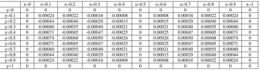
Table 2. Values of the function u (x, y , t ) (elimination method) at t = 0.08

x=0 x=0.1 x=0.2 x=0.3 x=0.4 x=0.5 x=0.6 x=0.7 x=0.8 x=0.9 x=1

y=0 0 0 0 0 0 0 0 0 0 0 0

y=0.1 0 -0.00024 -0.00022 -0.00016 -0.00008 0 0.00008 0.00016 0.00022 0.00024 0 y=0.2 0 -0.00044 -0.00040 -0.00029 -0.00015 0 0.00015 0.00029 0.00040 0.00044 0 y=0.3 0 -0.00060 -0.00055 -0.00040 -0.00021 0 0.00021 0.00040 0.00055 0.00060 0 y=0.4 0 -0.00071 -0.00065 -0.00047 -0.00025 0 0.00025 0.00047 0.00065 0.00071 0 y=0.5 0 -0.00074 -0.00068 -0.00050 -0.00026 0 0.00026 0.00050 0.00068 0.00074 0 y=0.6 0 -0.00071 -0.00065 -0.00047 -0.00025 0 0.00025 0.00047 0.00065 0.00071 0 y=0.7 0 -0.00060 -0.00055 -0.00040 -0.00021 0 0.00021 0.00040 0.00055 0.00060 0 y=0.8 0 -0.00044 -0.00040 -0.00029 -0.00015 0 0.00015 0.00029 0.00040 0.00044 0 y=0.9 0 -0.00024 -0.00022 -0.00016 -0.00008 0 0.00008 0.00016 0.00022 0.00024 0

(6)

Table 3. Values of the function v (x, y , t ) (explicit scheme) at t = 0.08

x=0 x=0.1 x=0.2 x=0.3 x=0.4 x=0.5 x=0.6 x=0.7 x=0.8 x=0.9 x=1

y=0 0 0 0 0 0 0 0 0 0 0 0

y=0.1 0 -0.00039 -0.00072 -0.00099 -0.00117 -0.00123 -0.00117 -0.00099 -0.00072 -0.00039 0 y=0.2 0 -0.00034 -0.00064 -0.00089 -0.00104 -0.00109 -0.00104 -0.00089 -0.00064 -0.00034 0 y=0.3 0 -0.00025 -0.00047 -0.00064 -0.00076 -0.00080 -0.00076 -0.00064 -0.00047 -0.00025 0 y=0.4 0 -0.00013 -0.00025 -0.00034 -0.00040 -0.00042 -0.00040 -0.00034 -0.00025 -0.00013 0

y=0.5 0 0 0 0 0 0 0 0 0 0 0

y=0.6 0 0.00013 0.00025 0.00034 0.00040 0.00042 0.00040 0.00034 0.00025 0.00013 0 y=0.7 0 0.00025 0.00047 0.00064 0.00076 0.00080 0.00076 0.00064 0.00047 0.00025 0 y=0.8 0 0.00034 0.00064 0.00089 0.00104 0.00109 0.00104 0.00089 0.00064 0.00034 0 y=0.9 0 0.00039 0.00072 0.00099 0.00117 0.00123 0.00117 0.00099 0.00072 0.00039 0

y=1 0 0 0 0 0 0 0 0 0 0 0

Table 4. Values of the function v (x, y , t ) (elimination method) at t = 0.08

x=0 x=0.1 x=0.2 x=0.3 x=0.4 x=0.5 x=0.6 x=0.7 x=0.8 x=0.9 x=1

y=0 0 0 0 0 0 0 0 0 0 0 0

y=0.1 0 -0.00039 -0.00072 -0.00099 -0.00117 -0.00123 -0.00117 -0.00099 -0.00072 -0.00039 0 y=0.2 0 -0.00034 -0.00065 -0.00089 -0.00104 -0.00110 -0.00104 -0.00089 -0.00065 -0.00034 0 y=0.3 0 -0.00025 -0.00047 -0.00065 -0.00076 -0.00080 -0.00076 -0.00065 -0.00047 -0.00025 0 y=0.4 0 -0.00013 -0.00025 -0.00034 -0.00040 -0.00042 -0.00040 -0.00034 -0.00025 -0.00013 0

y=0.5 0 0 0 0 0 0 0 0 0 0 0

y=0.6 0 0.00013 0.00025 0.00034 0.00040 0.00042 0.00040 0.00034 0.00025 0.00013 0 y=0.7 0 0.00025 0.00047 0.00065 0.00076 0.00080 0.00076 0.00065 0.00047 0.00025 0 y=0.8 0 0.00034 0.00065 0.00089 0.00104 0.00110 0.00104 0.00089 0.00065 0.00034 0 y=0.9 0 0.00039 0.00072 0.00099 0.00117 0.00123 0.00117 0.00099 0.00072 0.00039 0

y=1 0 0 0 0 0 0 0 0 0 0 0

Table 5. Values of the function T (x, y , t ) (explicit scheme) at t = 0.08

x=0 x=0.1 x=0.2 x=0.3 x=0.4 x=0.5 x=0.6 x=0.7 x=0.8 x=0.9 x=1

y=0 15 15 15 15 15 15 15 15 15 15 15

y=0.1 15 16.40181 17.66636 18.66994 19.31427 19.53630 19.31427 18.66994 17.66636 16.40181 15 y=0.2 15 17.66627 20.07145 21.98024 23.20575 23.62804 23.20575 21.98024 20.07145 17.66627 15 y=0.3 15 18.66981 21.98023 24.60743 26.29420 26.87542 26.29420 24.60743 21.98023 18.66981 15 y=0.4 15 19.31412 23.20574 26.29420 28.27710 28.96036 28.27710 26.29420 23.20574 19.31412 15 y=0.5 15 19.53613 23.62803 26.87542 28.96036 29.67879 28.96036 26.87542 23.62803 19.53613 15 y=0.6 15 19.31412 23.20574 26.29420 28.27710 28.96036 28.27710 26.29420 23.20574 19.31412 15 y=0.7 15 18.66981 21.98023 24.60743 26.29420 26.87542 26.29420 24.60743 21.98023 18.66981 15 y=0.8 15 17.66627 20.07145 21.98024 23.20575 23.62804 23.20575 21.98024 20.07145 17.66627 15 y=0.9 15 16.40181 17.66636 18.66994 19.31427 19.53630 19.31427 18.66994 17.66636 16.40181 15

y=1 15 15 15 15 15 15 15 15 15 15 15

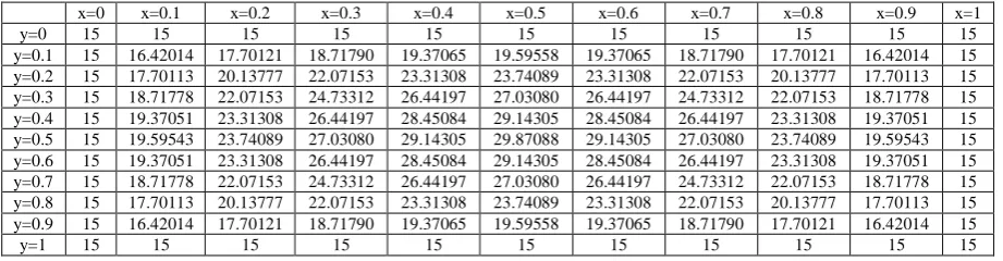
Table 6. Values of the function T (x, y , t ) (elimination method) at t = 0.08

x=0 x=0.1 x=0.2 x=0.3 x=0.4 x=0.5 x=0.6 x=0.7 x=0.8 x=0.9 x=1

y=0 15 15 15 15 15 15 15 15 15 15 15

y=0.1 15 16.42014 17.70121 18.71790 19.37065 19.59558 19.37065 18.71790 17.70121 16.42014 15 y=0.2 15 17.70113 20.13777 22.07153 23.31308 23.74089 23.31308 22.07153 20.13777 17.70113 15 y=0.3 15 18.71778 22.07153 24.73312 26.44197 27.03080 26.44197 24.73312 22.07153 18.71778 15 y=0.4 15 19.37051 23.31308 26.44197 28.45084 29.14305 28.45084 26.44197 23.31308 19.37051 15 y=0.5 15 19.59543 23.74089 27.03080 29.14305 29.87088 29.14305 27.03080 23.74089 19.59543 15 y=0.6 15 19.37051 23.31308 26.44197 28.45084 29.14305 28.45084 26.44197 23.31308 19.37051 15 y=0.7 15 18.71778 22.07153 24.73312 26.44197 27.03080 26.44197 24.73312 22.07153 18.71778 15 y=0.8 15 17.70113 20.13777 22.07153 23.31308 23.74089 23.31308 22.07153 20.13777 17.70113 15 y=0.9 15 16.42014 17.70121 18.71790 19.37065 19.59558 19.37065 18.71790 17.70121 16.42014 15

(7)

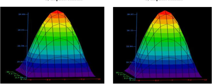
a) Explicit scheme b) Implicit scheme

Fig. 1 a, b. Distribution of displacement u (x, y, t) in an orthotropic rectangle with

t



0.08

a) Explicit scheme b) Implicit scheme

Fig. 2 a, b. Distribution of displacement v (x, y , t) in an orthotropic rectangle with

t



0.08

a) Explicit scheme b) Implicit scheme

(8)

CONCLUSION

Tables 1-6 show the numerical results of a two-dimensional coupled dynamic problem of an orthotropic rectangle. According to the initial and boundary conditions ( 22), a clamped rectangle is initially applied with a temperature field. The elastic constants of an orthotropic material are slightly different from an isotropic material. Deforming process mainly comes from - the thermal field. According to tables 5-6, you can see that the highest temperature is reached in the center of the rectangle and pa , but, respectively, 29.679 and 29.871 according to the explicit scheme and the elimination method. From Tables 1–4, it can be seen that the displacement values obtained by the two mentioned methods almost coincide; this ensures the validity of the numerical results obtained.

REFERENCES

[1] Biot M.A. Thermoelasticity and Irreversible thermodynamics. J. of Appl. Physics. Vol. 27, №3, p.240-253, 1956

[2] Lord H.W. and Shulman Y., (1967). A generalized dynamical theory of thermoelasticity,J. Mech. Phys. Solids, Vol. 15 (5), pp. 299-309.

[3] Muller, I.M.: The coldness, a universal function in thermoelastic bodies. ¨ Arch. Rational Mech. Anal., 319, (1971), 41.

[4] Youssef H.M. Theory of two-temperature-generalized thermoelasticity. IMA J. of APPL. Math. 2006, 71, p.383-390

[5] Aboudi J. The effective thermomechanical behavior of inelastic fiber-reinforced materials. Int. J. Engng. Sci., 1985. 23, No 7. - P. 773-787,

[6] Nowacki W., Dynamic problems of thermoelasticity, M.Mir, 1970, 256 p. (in Russian)

[7] Samarskii A., Nikolaev E. Numerical methods of grid equation, Birkhauser Verlag, Berlin, 1989.

[8] Khaldjigitov A., Qalandarov A., Nik M.A.Asri Long, Eshquvatov Z. Numerical solution of 1D and 2D thermoelastic coupled problems. International journal of modern physics. Vol. 9, pp. 503-510, 2012.

AUTHORS PROFILE

Kalandarov Aziz Abdukayumovich

He graduated from magistracy at National University of Uzbekistan. PhD on physical and mathematical science. Conducts research in the field of mathematical and numerical modeling of thermo-elastic-plastic processes. E-mail: [email protected].

Babadjanov Mumin Radjabovich