cuHE: A Homomorphic Encryption Accelerator Library
Wei Dai and Berk Sunar
Worcester Polytechnic Institute, Worcester, Massachusetts, USA
Abstract. We introduce a CUDA GPU library to accelerate evaluations with homomorphic schemes defined over polynomial rings enabled with a number of optimizations including algebraic techniques for efficient evaluation, memory minimization techniques, memory and thread scheduling and low level CUDA hand-tuned assembly optimizations to take full advantage of the mass parallelism and high memory bandwidth GPUs offer. The arithmetic functions constructed to handle very large polyno-mial operands using number-theoretic transform (NTT) and Chinese remainder theorem (CRT) based methods are then extended to implement the primitives of the leveled homomorphic encryption scheme proposed by L´opez-Alt, Tromer and Vaikuntanathan. To compare the performance of the proposed CUDA library we implemented two applications: the Prince block cipher and homomorphic sorting algorithms on two GPU platforms in single GPU and multiple GPU configurations. We observed a speedup of 25 times and 51 times over the best previous GPU implementation for Prince with single and triple GPUs, respectively. Similarly for homomorphic sorting we obtained 12-41 times speedup depending on the number and size of the sorted elements.
Keywords:Homomorphic evaluation, GPU acceleration, large polynomial arithmetic.
1 Introduction
Fully homomorphic encryption (FHE) has gained increasing attention from cryptographers ever since its first plausible secure construction was introduced by Gentry [17] in 2009. FHE allows one to perform arbitrary computation on encrypted data without the need of a secret key, hence without knowledge of original data. That feature would have invaluable implications for the way we utilize computing services. For instance, FHE is capable of protecting the privacy of sensitive data on cloud computing platforms. We have witnessed amazing number of improvements in fully and somewhat homomorphic encryption schemes (SWHE) over the past few years [20, 34, 3, 4, 18, 2]. In [19] Gentry, Halevi and Smart (GHS) proposed the first homomorphic evaluation of a complex circuit, i.e. a full AES block. The implementation makes use of batching [31, 32], key switching [2] and modulus switching techniques to efficiently evaluate a leveled circuit. In [28] a leveled NTRU [24, 33] based FHE scheme was introduced by L´opez-Alt, Tromer and Vaikuntanathan (LTV), featuring much slower growth of noise during homomorphic computation. Later Dor¨oz, Hu and Sunar (DHS) [11] used an LTV SWHE variant to evaluate AES more efficiently. More recently, Ducas and Micciancio [15] presented an efficient implementation of the bootstrapping algorithm.
to homomorphically evaluate dynamic programming algorithms such as Hamming distance, edit distance, and the Smith-Waterman algorithm on encrypted genomic data. C¸ etin et al. [6] analyzed the complexity and provided implementation results for homomorphic sorting.
Despite the rapid advances, HE evaluation efficiency remains as one of the obstacles preventing it from deployment in real-life applications. Given the computation and bandwidth complexity of HE schemes, alternative platforms such as FPGAs, application-specific integrated circuits (ASIC) and graphics processor units (GPU) need to be employed. Over the last decade GPUs have evolved to highly parallel, multi-threaded, many-core processor systems with tremendous computing power. Compared to FPGA and ASIC platforms, general-purpose computing on GPUs (GPGPU) yields higher efficiency when normalized by price. For example, in [12] an NTT conversion costs 0.05 msec on a $5,000 FPGA, whereas takes only 0.15 msec on a $200 GPU (NVIDIA GTX 770). The results of [35, 9, 10] demonstrate the power of GPU-accelerated HE evaluations. Another critical advantage of GPUs is the strong memory architecture and high communication bandwidth. Bandwidth is crucial for HE evaluation due to very large evaluation keys and ciphertexts. In contrast, FPGAs feature much simpler and more limited memory architectures and unless supplied with a custom memory I/O interface design the bandwidth suffers greatly.
For CPU platforms Halevi and Shoup published the HElib [23], a C++ library for HE that is based on Brakerski-Gentry-Vaikuntanathan (BGV) cryptosystem [2]. More recently, Ducas and Micciancio [15] published FHEW, another CPU library which features encryption and bootstrap-ping. In this paper, we propose cuHE: a GPU-accelerated optimized SWHE library in CUDA/C++. The library is designed to boost polynomial based HE schemes such as LTV, BGV and DHS. Our aim is to accelerate homomorphic circuit evaluations of leveled circuits via CUDA GPUs. To demon-strate the performance gain achieved with cuHE, by employing the DHS scheme [11], along with many optimizations, to implement the Prince block cipher and a homomorphic sorting algorithm on integers.
Our Contributions
– The cuHE library offers the feasibility of accelerating polynomial based homomorphic encryption and various circuit evaluations with CUDA GPUs.
– We incorporated various optimizations and design alternative methods to exploit the memory organization and bandwidth of CUDA GPUs. In particular, we adapted our parameter selection process to optimally map HE evaluation keys and precomputed values into the right storage type from fastest and more frequently used to slowest least accessed. Moreover, we also utilized OpenMP and CUDA hybrid programming for simultaneous computation on multiple GPUs.
– We attain the fastest homomorphic block cipher implementation, i.e. Prince at 51 msec (1 GPU), using the cuHE library which is 25 times faster than the previously reported fastest implementation [9]. Further, our library is able to evaluate homomorphic sorting on an integer array of various sizes 12-41 times faster compared to a CPU implementation [6].
2 Background
2.1 The LTV SWHE Scheme
In this section we briefly explain the LTV SWHE [28] with specializations introduced in [11]. We work with polynomials in ring R = Z[x]/(m(x)) where degm(x) = n. All operations are
of {b−2qc, . . . ,b2qc}. A truncated discrete Gaussian distribution χ is used as an error distribution from which we can sample random smallB-bounded polynomials. The primitives of the public key encryption scheme are Keygen,Enc,Dec and Eval.
Keygen We generate a decreasing sequence of odd moduli q0 > q1 > · · · > qd−1 where d denotes
the circuit depth and a monic polynomial m(x). They define the ring for each level. m(x) is the product of l monic polynomials each of which defines a message slot. In [11] more details about batching are explained. Keys are generated for the 0-th level, and are updated for every other level. The 0-th level Sample α, β ← χ, and set sk(0) = 2α + 1 and pk(0) = 2β(sk(0))−1 in ring Rq0 =Zq0[x]/hmi(re-sample ifsk
(0) is not invertible in the this ring). Then for τ ∈
Zdlogq0
w e
where
w6logqd−1is a preset value, samples(0)τ , e(0)τ ←χand publish evaluation key{ek(0)τ |τ ∈Zdlogq0
w e
}
where ek(0)τ = pk(0)s(0)τ + 2e(0)τ + 2wτsk(0). The i-th level Compute sk(i) = sk(0) (mod qi) and
pk(i)=pk(0) (modqi) in ringRqi =Zqi[x]/hmi. Then compute evaluation key {ek (i)
τ |τ ∈Zdlogqi
w e
}
whereekτ(i)=ek(0)τ (modqi).
Enc To encrypt a bit b ∈ {0,1} with public key (pk(0), q
0), sample s, e ← χ, and set c(0) = pk(0)s+ 2e+binRq0.
Dec To decrypt a ciphertext c(i), multiply the ciphertext with the corresponding private keysk(i) inRqi and then compute the message by modulo two:b=c
(i)sk(i) (mod 2).
EvalWe perform arithmetic operations directly on ciphertexts. Supposec(1i)=Enc(b1) (modqi) and
c(2i) =Enc(b2) (modqi). TheXORgate is realized by adding ciphertexts: b1+b2 =Dec(c(1i)+c (i) 2 ).
The AND gate is realized by multiplying ciphertexts. However, polynomial multiplication incurs a much greater growth in the noise. So each multiplication step is followed by relinearization and modulus switching. First we compute ˜c(i)=c(i)
1 ×c
(i)
2 inRqi. To obtain ˜c
(i+1) from ˜c(i), we perform
relinearization on ˜c(i). We expand it as ˜c(i) =Pd logqi
w e
τ=0 2τ˜c (i)
τ where ˜c(τi) takes its coefficients from
Z2w. Then set ˜c(i+1) = P
dlogqi
w e
τ=0 ek (i)
τ ˜c(τi) in Rqi. To obtain c
(i+1) in R
qi+1, we perform modulus switching: c(i+1) =bqi+1
qi c (i)e
2 and then we have m1×m2=Dec(c(i+1)).
2.2 Arithmetic Tools
Sch¨onhage-Strassen’s Multiplication Here we very briefly introduce Sch¨onhage-Strassen’s polynomial multiplication scheme [29]. Given f = Pn−1
k=0akxk and g = Pkn−=01bkxk, we compute
ˆ
f =P2n−1
k=0 ˆakxk, where [ˆa0,aˆ1, . . . ,aˆ2n−1] =NTT([a0, a1, . . . , an−1,0, . . . ,0]). One multiplication of
two degree n polynomials consists of two 2n-point NTTs, one coefficient-wise multiplication and one 2n-point inverse transform (INTT):
– Inputs:f =Pn−1
k=0akxk,g=Pkn=0−1bkxk; – NTT Conversion: f →fˆ=P2n−1
k=0 aˆkxk,g→ˆg=P2kn=0−1ˆbkxk; – Output: f ×g=INTT(P2n−1
k=0 ˆakˆbkxk).
CRT We introduce the CRT to handle large integer computation. We generate t prime numbers {p0, p1, . . . , pt−1} with Bp < 32 bits. We further compute, for each level, qi = p0p1· · ·pti where
Pn−1
k=0akxk in ring Rqi, we compute a vector of polynomials F = [f(0), f(1), . . . , f(ti−1)] as its
CRT representation: f(j) = Pn−1
k=0ak(j)xk ∈ Rpj, where ak(j) = ak (mod pj), j ∈ Zti. For all
f, g ∈ Rqi where i ∈ Zd, and F = CRT(f), G = CRT(g), we have f ◦g = ICRT(F ◦ G), where
F ◦ G = [f(0)◦g(0), . . . , f(ti−1)◦g(ti−1)]. Given a polynomial modulusmandM=CRT(m), for allf,
we havef (modm) =ICRT(F (mod M)). Other than CRT and ICRT, no large integer operation is needed.
2.3 CRT, NTT
In our implementations, the degree of modulus m is 8192, 16384 or 32768. Andq0 has more than
256, 512 or 1024 bits, respectively. Coefficient independent operations, e.g. polynomial addition, can provide sufficient parallelism for a GPU realization. Still, two problems remain to be solved: how to compute large integers on CUDA GPUs; and how to efficiently implement operations that are not coefficient independent, e.g. polynomial multiplication. Those problems are handled by using CRT and NTT together.
3 GPU Basics
GPUs are powerful but highly specialized devices that require careful coding to take full advantage of the massive parallelism offered. Specifically, the programming model and memory organization is much different from in CPUs. Here we present a concise overview.
3.1 Programming Model
In general, a GPU-accelerated scheme offloads compute-intensive portions of the application to the GPU, while the remainder of the code still runs on the CPU. A GPU has its own on-chip memory. We call the CPU and memory “host”, while GPU and its on-chip memory “device”. A normal GPU computational task includes 3 operations: copying essential data from host to device (memcpy h2d), initializing computation (akernel) on device, copying result from device to host (memcpy d2h) when necessary. A CUDA kernel is executed by an array of sequential threads. All threads run the same code, with an ID to compute memory addresses and make control decisions. On a GPU with warp size of 32, the kernel is executed in groups of 32 threads. Threads are further grouped into blocks. Only threads within a block can cooperate or synchronize. A kernel launch defines a grid of thread blocks. The dimension of a grid and that of each block determine how computing resource is assigned to program. The computation complexity of a kernel and the amount of data transferred between host and device depend on the details of an implementation.
3.2 Stream Management
kernel execution. Alternatively, we may further break down one kernellaunch into several parts in order to create concurrency. Every stream belongs to its own device. To have streams on different devices run concurrently and synchronize as needed is multi-GPU computing. However, merely using streams to launch tasks on different devices creates expensive latency. Using OpenMP along with streams is a better solution. The goal of stream management is to achieve the best possible utilization of computing resources.
3.3 Memory Management
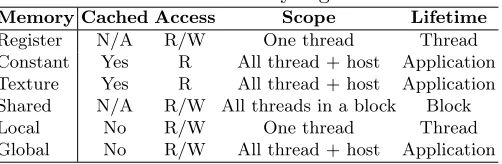
A significant ingredient to the performance of a program is memory management. The effect is particularly strong on GPUs since there are many different types of memory to store data and since the GPU-CPU interface tends to be slow. The GPU memory architecture is represented in Table 5 (see Appendix). Memory types are listed from top to bottom by access speed from fast to slow. Before executing a kernel, we need to feed constant memory and global memory with data, and bind texture memory if needed. Other than using streams to overlap data transfer and computation, we optimize these data transfers in following methods: minimizing the amount of data transferred between host and device when possible, batching many small transfers into one larger transfer, using page-locked (or pinned) memory to achieve a higher bandwidth. Towards an efficient application,kernels should be designed to take advantage of the memory hierarchy properties:
– Constant memory is cached and fast. Due to its limited size, e.g. 64 KB, it is only suitable for repeatedly requested data.
– Global memory is not cached, expensive to access, and huge in size, e.g. 2 GB. Data that is only read once, or is updated by kernels is better allocated in global memory. The pattern of memory access in kernels also matters. If each thread in a warp accesses memory contiguously from the same 128 B chunk, it is called coalesced memory access. A non-coalesced (strided) memory access could make a kernelhundreds of times slower.
– Texture memory is designed for this scenario: a thread is likely to read from an address near the ones that nearby threads read (non-coalesced). It is better to use texture memory when the data is updated rarely but read often, especially when the read access pattern exhibits a spatial locality.
– Shared memory is allocated for all threads in a block. It offers better performance than local or global memory and allows all threads in a block to communicate. Thus it is often used as a buffer to hold intermediate data, or to re-order strided global memory accesses to a coalesced pattern. However, only a limited size of shared memory can be allocated per block. Typically one configures the number of threads per block according to shared memory size. The shared memory is accessed by many threads, so that it is divided into banks. Since each bank can serve only one address per cycle, multiple simultaneous accesses to a bank result in a bank conflict. If all threads of a half-warp access a different bank (no bank conflict), the shared memory may become as fast as the registers.
4 Our Contribution: A CUDA Polynomial Arithmetic Library
It has 1536 CUDA cores, 2 GB memory, 64 KB constant memory, 48 KB shared memory per block, CUDA Capability 3.0 and warp size of 32. On a device with better specifications, the program is believed to provide a better performance, yet has room to improve if configured and customized for the device.
4.1 Overview
Interfacing with NTL. We build our library to interface with the NTL library by Shoup [30]. Most implementations of polynomial based HE schemes are built on NTL. We provide an interface to NTL data types, in particular to the polynomial class ZZX so that GPU acceleration can be achieved with very little modification to a program. Another reason is that we only support very limited types of polynomial operations. Therefore, until non performance critical operations, e.g. a polynomial inversion in a polynomial ring, are implemented we may still utilize the NTL library.
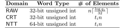
Polynomial Representation. Suppose we work within the i-th level of a circuit. To store an
Table 1: Polynomial Representation on a GPU.
Domain Word Type # of Elements
RAW 32-bit unsigned int ndlogqi
32 e
CRT 32-bit unsigned int tin NTT 64-bit unsigned int tin
n-degree polynomial inRqi in GPU memory, we use an array of nd logqi
32 e 32-bit unsigned integers,
where every dlogqi
32 e integers denote a polynomial coefficient. We call a polynomial of this form in
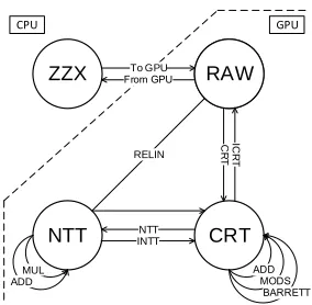
RAW domain. In the background section, we introduced two techniques: CRT and NTT, which give a polynomial CRT and NTT domain representations. Table 1 lists the structure and storage size of a polynomial in each domain. Figure 1 illustrates basic routines of operations on polynomials. Due to mathematical properties, each domain supports certain operations more efficiently as shown in Figure 1. In other words, to perform a certain operation, the polynomial should first be converted to a specific domain unless it is already in the desired domain. As shown in Table 1, the CRT domain representation requires more space than the RAW domain. However, having polynomials stay in the CRT domain saves one CRT conversion in every polynomial operation and one ICRT conversion in every operations except relinearization. Moreover, the sequence of operations might also create unnecessary latency if there are conversions that could have been spared.
4.2 CRT/ICRT
CRT prime numbers are precomputed based on the application settings and are stored in constant memory. ICRT conversion for a coefficientxisx=Pti−1
j=0 qi/pj·((qi/pj)
−1·x
(j) (modpj)) (modqi)
whereqi =Qjti=0−1pj. To efficiently compute ICRT, constants:qi,{pqij}and{(pqij)−1(modpj)}, where
j ∈ Zti, are also precomputed and stored in constant memory. Given the coefficients of a RAW
domain polynomial [a0, . . . ,an−1], the number of 32-bit unsigned integers we use to represent each coefficient ak ∈ Zqi is |ak| =d
logqi
32 e. Its CRT domain representation is {[a0(j), . . . ,an−1(j)]|j ∈
RAW
CRT NTT
RAW ZZX
MUL ADD
RELIN
C
R
T
IC
R
T
NTT INTT To GPU
GPU CPU
Fig. 1: Four representation domains for polynomials
ak, as in Figure 4a (see Appendix). However, that exhibits strided global memory access. Instead, we use shared memory to build a buffer as in Figure 4b (see Appendix). Not only do we reorder all accesses to global memory as coalesced, but also we avoid bank conflicts when reading or writing to shared memory. TheICRT kerneloperation is designed similarly. Moreover, we make wide use of registers in ICRT kernelwith assembly code for a better performance.
4.3 NTT/INTT
NTT is performed on a polynomial inRpj. We take an arrayA= [a0, . . . , an−1,0, . . . ,0], i.e.n
coef-ficients appended with nzeros, as input. We obtain a new array ˆA= [ˆa0, . . . ,ˆa2n−1] by performing
a 2n-point NTT on A. Given ti CRT prime numbers, to convert a CRT domain polynomial to
NTT domain, we need ti NTTs. We follow the approach of Dai et al. [9] to build an NTT scheme
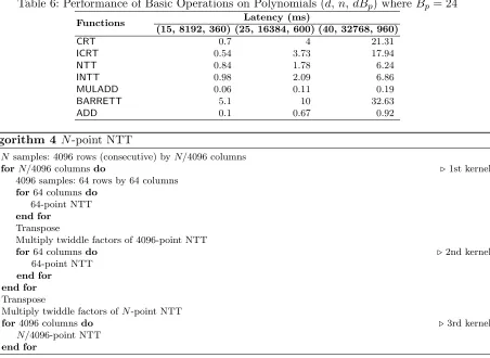
on GPU. According to FHE scheme settings, we only support NTTs of 16384, 32768 and 65536 points. LetN = 2n be the size of NTT. We construct three CUDA kernels to adopt the four-step Cooley-Tukey algorithm [8]. As shown in Algorithm 4 (see Appendix), an N-point NTT is com-puted with several smaller size NTTs. What is not shown in Algorithm 4 is that a 64-point NTT is computed with 8-point NTTs. In [16] the benefit of working in finite field FP is demonstrated
whereP =0xFFFFFFFF00000001. In such a field, moduloP operations may be computed efficiently. Besides, 8 is a 64-th primitive root ofP. By usingh8i ⊂FP, 64-point NTTs can be done with shifts
rather than requiring 64-bit by 64-bit multiplications. We build inline device functions for arith-metic operations in FP in assembly code. In kernels we use shared memory to store those points.
That ensures coalesced global memory accesses and fast transpose computation. We precompute 2N twiddle factors and bind them to texture memory since they are constant and are too large for constant memory. INTT is basically an NTT with extra steps. Given ˆA= [ˆa0, . . . ,ˆa2n−1], we first
re-order the array as ˆA0 = [ˆa0,aˆ2n−1,aˆ2n−2, . . . ,aˆ1]. Then we compute A= N1NTT( ˆA
0
) (modpj).
4.4 Polynomial Multiplication
Algorithm 1 Polynomial Multiplication
1: Input NTT domain polynomials ˆF and ˆG
2: ˆH= ˆF ·Gˆ .coefficient-wise multiplication
3: H ←INTT( ˆH) .convert to CRT domain
4: OutputH(modM) .polynomial modular reduction
INTTs,DOTMUL is almost negligible in terms of overhead. Since the product is a (2n−2)-degree polynomial in CRT domain, it is followed by modular reductions overRpj, for allj ∈Zt.
4.5 Polynomial Addition
Polynomial addition is essential for two functions in homomorphic circuit evaluation. One is in the homomorphic evaluation of an XOR gate which is simply implemented as a polynomial addition. For this the addition operation is carried out in the CRT domain. It provides sufficient parallelism for a GPU to process and also yields a result in the ringRqi without the need of coefficient modular
reduction. The other computation that needs polynomial addition is in the accumulation part of relinearization. We will discuss this in detail later.
4.6 Polynomial Barrett Reduction
Polynomial computation is in ring Rqi =Zqi/m, where degm =n. Given a computation resultf
with degf >n, a polynomial reduction modulom is needed. In fact, degf ≤2n−2 always holds in our construction. We implement a customized Barrett reduction on polynomials by using our polynomial multiplication schemes as in Algorithm 2. We precomputed all constant polynomials generated from the modulus, and stored them in the GPU memory as described in the procedure “Precomputation”. The goal of Barrett reduction is to computer=f (modm). We take the CRT domain polynomial as input and return CRT domain polynomial as output.
4.7 Supporting HE Operations
To evaluate a leveled circuit, besides operations introduced above, we need other processes to reduce the introduced noise, e.g. by multiplication. An AND gate is followed by a relinearization. All ciphertexts are processed with modulus switching to be ready for next level. In our implementation Keygen is modified for a faster relinearization and parameters are selected to accommodate our GPU implementation.
Relinearization.A relinearization computes products of ciphertexts and evaluation keys. It then accumulates the products. By operating additions in the NTT domain we reduce the overhead of INTT in each multiplication. Given a polynomialc(i)in RAW domain we first expand it to ˜c(τi)where
τ ∈ Zηi and ηi =d logqi
w e. We call w the size of relinearization window. Then we need to compute
˜ c(i+1) =
ηi
X
τ=0
ekτ(i)˜cτ(i) in Rqi which is equivalent to computing ˜C
(i+1) = INTT
ηi
X
τ=0
ˆ EK(τi)Cˆ˜τ(i)
. We
find a way to precompute and store evaluation keys for all levels. InKeygen, we convert evaluation keys of the 0-th level to NTT domain and store them. For everyτ ∈Zη0 compute
Algorithm 2 Polynomial Barrett Reduction
1: procedurePrecomputation(m) 2: u=bx2n−1/mc
3: StoreM=CRT(m) 4: Store ˆM=NTT(M) 5: Store ˆU=NTT(CRT(u)) 6: end procedure
7: procedureBarrettReduction(F)
8: Q=trunc(F, n−1) .input in CRT domain
9: Qˆ=NTT(Q) .1st multiplication
10: Qˆ= ˆQ ∗Uˆ
11: Q=INTT( ˆQ) 12: Q=trunc(Q, n)
13: Qˆ=NTT(Q) .2nd multiplication
14: Qˆ= ˆQ ∗Mˆ
15: Q=INTT( ˆQ)
16: R=F − Q .subtraction
17: if degR>degMthen 18: R=R − M
19: end if
20: ReturnR .output in CRT domain
21: end procedure
Then{EKˆ (0)τ |τ ∈Zη0}is stored in GPU global memory. We no longer need to update the evaluation
keys for any other level, observing that ˆEK(τi)⊆EKˆ (0)τ , for alli∈Zdandτ ∈Zηi. Here what matters
the most is the overhead of expanding and converting the ciphertexts. To convert ˜c(τi) toCˆ˜τ(i) for all
τ ∈ Zηi, we need ηi CRTs and ηiti NTTs. However, if we set w < logpj, then for all j ∈ Zt0 we have ˜c(τi)∈R2w ⊂Rp
j, i.e. ˜C (i)
τ ={˜c(τi)}. In such a setting, we only need ηi NTTs to convert ˜c(τi) to
the NTT domain.
Based on these optimizations, we build a multiplier and accumulator for NTT domain polyno-mials. Suppose we have sufficient memory on GPU to hold all ˆEK(0)τ . Only one kernelthat uses the
shared memory to load allCˆ˜τ(i) will suffice. We also provide solutions when the evaluation keys are
too large for the GPU memory to hold. On a multi-GPU system, we evenly distribute the keys on devices. When the keys on another device is requested, copy them from that device to the current device. This is the best solution for two reasons: the bandwidth between devices is much larger than that between the device and host; accesses to memory on another device in akernel yield roughly 3 times less overhead, compared to accessing the current device’s memory.
Double-CRT Setting.According to [11], to correctly evaluate a circuit of depthdand to reach a desired security level, we can determine the lower bounds of nand logq0, and thatδq ≤logqiq+1i =
Qti−1
j=tipj wherei∈Zd. Let Bp be the size of CRT prime numbers, i.e. Bp = logpj. Then we know
that 2Bp <pP/n <232. To simplify, we set t
i=d−i−1,Bp ≥δq. Then we have
δq ≤Bp <log
p P/n.
We selectBp =δq. Then we select the relinearization window size such asw < Bp. In these settings,
Algorithm 3 Modulus Switching
1: A={a(0), . . . , a(ti−1)} ←CRT(a
(i))
2: fork←1,do 3: a∗←a(ti−k)
4: if a∗= 1 (mod 2)then 5: if a∗>(pti−k−1)/2then 6: a∗=a∗−pti−k
7: else
8: a∗=a∗+pti−k 9: end if
10: end if
11: A= (A −a∗)/pti−k(modpti−k) 12: end for
13: a(i+1)=ICRT(A) =ICRT {a
(0), . . . , a(ti+1−1)}
Modulus Switching. In [19] Gentry et al. proposed a method to perform modulus switching on ciphertexts in CRT domain (double-CRT), by generating qi = p0p1· · ·pti−1 where i ∈ Zd.
Since modulus switching is a coefficient independent operation, to simplify, we represent it on a single coefficient. Given a coefficient a(i) ∈
Zqi where i∈Zd, modulus switching is designed as in
Algorithm 3 to obtain a(i+1) ∈ Zqi+1 such that a
(i+1) = a(i) (mod 2) and = |a(i+1) − qi+1
qi a (i)|
where −1 ≤≤1 always holds. We precomputep−j1 (modpk) for all k∈Zt0 \Ztd−1 and j ∈Zk. These values are stored as a lookup table in constant memory.
Precomputation Routine. For a circuit with depthd, we select parameters with a sequence of constraints: d → n → δq → Bp → w. We generate a set of d prime numbers with Bp bits P =
{p0, . . . , pd−1}as CRT constants. For each level i∈Zd of the circuit we generate ICRT constants:
qi =Qji−=01 pj, Q∗i ={ qi
pj |j ∈Zi} and Q
† i ={(
qi
pj)
−1 (mod p
j) |j∈Zi}. We also generate Modulus
Switching constants for all levels: P−1 = {p−1
j,k =p −1
k (modpj)|j∈Zi\ {0}, k∈Zj}. P and P −1
are stored in GPU constant memory. However, we store Q={qi |i∈Zd},Q∗ ={Q∗i |i∈Zd} and
Q† ={Q†
i |i∈Zd} in CPU memory at first. We update ICRT constants for ICRT conversions in
a new level by copying qi, Q∗i and Q †
i to GPU constant memory. We generate an n degree monic
polynomial m as polynomial modulus and compute u = x2n−1/m ∈ Rq0 for Barrett reduction. Their CRT and NTT domain representations M, Mˆ and ˆU are computed and bound to GPU texture memory. Table 2 is a summary of precomputed data, showing storage memory types and sizes. Besides general expressions of size in bytes, we also list the memory usage of three target circuits: Prince stands for the Prince block cipher that has [d= 25, n= 16384, Bp= 25, w= 16].
Sorting(8) is a sorting circuit of 8 unsigned 32-bit integers, with parameters set to [13, 8192, 20, 16]. Similarly, Sorting(32) sorts 32 unsigned integers and has parameters [15, 8192, 22, 16].
Keygen As explained in background, for all levels, we generate secret keys sk(i) and public keys pk(i). Based on those, we computeekτ(i) as evaluation keys. We then convert and store their NTT domain representations ˆEKτ(i) in GPU memory.
5 Implementation Results
Table 2: Precomputation
Content Memory Size (Bytes)
Type Equation Prince Sorting(8) Sorting(32)
P constant 4d 100 52 60
qi constant 4d(d−i)Bp/32e ≤80 ≤36 ≤44
Q∗
i constant 4(d−i)d(d−i−1)Bp/32e ≤1,900 ≤416 ≤600
Q†i constant 4(d−i) ≤100 ≤52 ≤60
P−1
constant 2d(d−1) 1,200 312 420
M texture 4dn 1,638,400 425,984 491,520
ˆ
M texture 16dn 6,553,600 1,703,936 1,966,080 ˆ
U texture 16dn 6,553,600 1,703,936 1,966,080 ˆ
EK(τi) global 16dnddBp/we 262,144,000 28,966,912 41,287,680
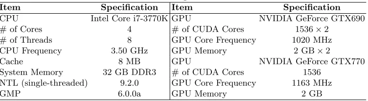
in both single GPU, i.e. GTX 680, and in multi-GPU modes. The testing environment is summarized in Table 3. We show performance of our library and compare it to CPU implementations using the NTL library (v9.2.0) which is adopted by DHS-HE [11] and HELib [22].
Table 3: Testing Environment
Item Specification Item Specification
CPU Intel Core i7-3770K GPU NVIDIA GeForce GTX690
# of Cores 4 # of CUDA Cores 1536×2
# of Threads 8 GPU Core Frequency 1020 MHz
CPU Frequency 3.50 GHz GPU Memory 2 GB×2
Cache 8 MB GPU NVIDIA GeForce GTX770
System Memory 32 GB DDR3 # of CUDA Cores 1536 NTL (single-threaded) 9.2.0 GPU Core Frequency 1163 MHz
GMP 6.0.0a GPU Memory 2 GB
5.1 Performance of GPU Library Primitives
Table 6 (see Appendix) shows the latency of the basic polynomial operations. MULADDstands for the multiplier and accumulator for NTT domain polynomials. ADD denotes polynomial addition in CRT domain. The latencies in the table of NTT conversions, whose speed is solely affected by n, consist ofditerations.
Figure 2a shows the performance of relinearization. Dor¨oz et al. [11] use the NTL library with an optimized polynomial reduction method. As shown in Figure 2b, the speedup is at least 20 times, and increases as the coefficient size increases, up to 160 times for 960 bit coefficients. Note that Dai et al. [9] did not fully implement relinearization on the GPU but rather relies on NTL/CPU for coefficient and polynomial reduction. For instance, for Prince parameters with coefficient size of 575 bits, our relinearization takes only 18.3 msec whereas Dai et al.’s takes 890 msec on GPU plus an additional 363 msec for reduction on the CPU. This yields a speedup of 68 times.
5.2 Performance of Sample Algorithms
(a) (b)
Fig. 2: Performance of relinearization (a) latency with growing coefficient size (b) speedup over [11]
Table 4: Performance of Implemented Algorithms
Platform Prince Sorting 8 Sorting 16 Sorting 32 Amortized
1/1024 Speedup
Amortized
1/630 Speedup
Amortized
1/630 Speedup
Amortized
1/630 Speedup
CPU (1-bit) [13] 3.3 sec 1 n/a n/a n/a n/a n/a n/a
GTX 680 (1-bit) [9] 1.28 sec 2.6 n/a n/a n/a n/a n/a n/a
CPU (16-bit) [13, 5] 1.98 sec 1.7 944 ms 1 4.28 sec 1 18.60 sec 1
GTX 680 (1 GPU) 51 ms 64 62 ms 15 291 ms 15 1.52 sec 12
GTX 770 (1 GPU) 45 ms 72 55 ms 17 256 ms 17 1.35 sec 14
GTX 690 (2 GPUs) 32 ms 103 34 ms 27 162 ms 26 864 ms 22
GTX 690/770 (3 GPUs) 24 ms 134 23 ms 41 108 ms 39 678 ms 27
evaluation performance is summarized in Table 4. We updated and reran Dor¨oz et al.’s homomorphic Prince [13] with a 16-bit relinearization window. With cuHE library, we achieve 40 times speedup on a single GPU, 135 times on three GPUs simultaneously, over the Dor¨oz et al. CPU implementation. Also compared to Dai et al.’s [9] the speedup is 25 times on the same GPU device.
Finally we would like to note that the proposed Prince implementation is thefastest homomor-phic block cipher implementation currently available. For instance, Lepoint and Naehrig evaluated homomorphic SIMON-64/128 in 2.04 sec with 4 cores on Intel Core i7-2600 at 3.4 GHz [27] for the n= 32,768 setting. Our homomorphic Prince is 40 times faster for n= 16,384, and 20 times for n= 32,768.
Acknowledgment
Appendix
memcpy_h2d (hd) memcpy_d2h (dh)
hd1 k1 dh2
hd2 k2 dh2
hd3 k3 dh3
hd4 k4 dh4
Speedup = 2 Single Stream Multiple Streams time time
hd1 k1 dh2 hd2 k2 dh2 hd3 k3 dh3 hd4 k4 dh4
Kernel (k)
Fig. 3: Improving performance by using multiple streams
T (0 ) T (0 ) T (0 ) ∙ ∙ ∙ T (1 ) T (1 ) T (1 ) ∙ ∙ ∙ ∙ ∙ ∙ T (d -1 ) T (d -1 ) T (d -1 ) ∙ ∙ ∙ ∙ ∙ ∙ Global Memory W /R Data
Block - d threads Strided
(a) T (1 ) T (0 ) T (d -1 ) ∙ ∙ ∙ T (1 ) T (0 ) ∙ ∙ ∙ T (1 ) T (0 ) T (d -1 ) ∙ ∙ ∙ ∙ ∙ ∙ ∙ ∙ ∙ Shared Memory Global Memory W /R Data syncthreads Coalesced
Block - d threads
T
(d
-1
)
(b)
Fig. 4: Using shared memory to avoid strided access to global memory.
Table 5: GPU memory organization
Memory Cached Access Scope Lifetime Register N/A R/W One thread Thread Constant Yes R All thread + host Application Texture Yes R All thread + host Application Shared N/A R/W All threads in a block Block
Local No R/W One thread Thread
Table 6: Performance of Basic Operations on Polynomials (d,n,dBp) whereBp = 24
Functions Latency (ms)
(15, 8192, 360) (25, 16384, 600) (40, 32768, 960)
CRT 0.7 4 21.31
ICRT 0.54 3.73 17.94
NTT 0.84 1.78 6.24
INTT 0.98 2.09 6.86
MULADD 0.06 0.11 0.19
BARRETT 5.1 10 32.63
ADD 0.1 0.67 0.92
Algorithm 4 N-point NTT
1: N samples: 4096 rows (consecutive) byN/4096 columns
2: forN/4096 columnsdo .1st kernel
3: 4096 samples: 64 rows by 64 columns 4: for64 columnsdo
5: 64-point NTT 6: end for
7: Transpose
8: Multiply twiddle factors of 4096-point NTT
9: for64 columnsdo .2nd kernel
10: 64-point NTT 11: end for
12: end for 13: Transpose
14: Multiply twiddle factors ofN-point NTT
15: for4096 columnsdo .3rd kernel
16: N/4096-point NTT 17: end for
References
1. Bos, J.W., Lauter, K., Naehrig, M.: Private predictive analysis on encrypted medical data. Tech. Rep. MSR-TR-2013-81 (September 2013), http://research.microsoft.com/apps/pubs/default.aspx?id=200652
2. Brakerski, Z., Gentry, C., Vaikuntanathan, V.: (leveled) fully homomorphic encryption without bootstrapping. In: Proceedings of the 3rd Innovations in Theoretical Computer Science Conference. pp. 309–325. ACM (2012) 3. Brakerski, Z., Vaikuntanathan, V.: Fully homomorphic encryption from ring-lwe and security for key dependent
messages. In: Advances in Cryptology–CRYPTO 2011, pp. 505–524. Springer (2011)
4. Brakerski, Z., Vaikuntanathan, V.: Efficient fully homomorphic encryption from (standard) lwe. SIAM Journal on Computing 43(2), 831–871 (2014)
5. C¸ etin, G.S., Dor¨oz, Y., Sunar, B., Sava¸s, E.: Low Depth Circuits for Efficient Homomorphic Sorting (To appear in LATINCRYPT 2015)
6. Chatterjee, A., Kaushal, M., Sengupta, I.: Accelerating sorting of fully homomorphic encrypted data. In: Paul, G., Vaudenay, S. (eds.) Progress in Cryptology INDOCRYPT 2013, Lecture Notes in Computer Science, vol. 8250, pp. 262–273. Springer International Publishing (2013)
7. Cheon, Jung, H., Miran, K., Kristin, L.: Secure dna-sequence analysis on encrypted dna nucleotides. (2014), http://media.eurekalert.org/aaasnewsroom/MCM/FIL 000000001439/EncryptedSW.pdf
8. Cooley, J.W., Tukey, J.W.: An algorithm for the machine calculation of complex Fourier series. Mathematics of computation 19(90), 297–301 (1965)
9. Dai, W., Dor¨oz, Y., Sunar, B.: Accelerating NTRU based Homomorphic Encryption using GPUs. 2014 IEEE High Performance Extreme Computing Conference (HPEC’14) (2014)
10. Dai, W., Dor¨oz, Y., Sunar, B.: Accelerating SWHE based PIRs using GPUs (To appear in WAHC’2015) 11. Dor¨oz, Y., Hu, Y., Sunar, B.: Homomorphic AES Evaluation using NTRU. IACR Cryptology ePrint Archive
12. Dor¨oz, Y., ¨Ozt¨urk, E., Sava¸s, E., Sunar, B.: Accelerating ltv based homomorphic encryption in reconfigurable hardware (To appear in Cryptographic Hardware and Embedded Systems–CHES 2015)
13. Dor¨oz, Y., Shahverdi, A., Eisenbarth, T., Sunar, B.: Toward practical homomorphic evaluation of block ciphers using prince. In: Financial Cryptography and Data Security, pp. 208–220. Springer (2014)
14. Dor¨oz, Y., Sunar, B., Hammouri, G.: Bandwidth efficient pir from ntru. In: B¨ohme, R., Brenner, M., Moore, T., Smith, M. (eds.) Financial Cryptography and Data Security, Lecture Notes in Computer Science, vol. 8438, pp. 195–207. Springer Berlin Heidelberg (2014)
15. Ducas, L., Micciancio, D.: Fhew: Bootstrapping homomorphic encryption in less than a second. In: Advances in Cryptology–EUROCRYPT 2015, pp. 617–640. Springer (2015)
16. Emmart, N., Weems, C.C.: High precision integer multiplication with a GPU using Strassen’s algorithm with multiple FFT sizes. Parallel Processing Letters 21(03), 359–375 (2011)
17. Gentry, C.: A fully homomorphic encryption scheme. Ph.D. thesis, Stanford University (2009)
18. Gentry, C., Halevi, S.: Fully homomorphic encryption without squashing using depth-3 arithmetic circuits. In: Foundations of Computer Science (FOCS), 2011 IEEE 52nd Annual Symposium on. pp. 107–109. IEEE (2011) 19. Gentry, C., Halevi, S., Smart, N.P.: Homomorphic evaluation of the AES circuit. In: Advances in Cryptology–
CRYPTO 2012, pp. 850–867. Springer (2012)
20. Gentry, C., et al.: Fully homomorphic encryption using ideal lattices. In: STOC. vol. 9, pp. 169–178 (2009) 21. Graepel, T., Lauter, K., Naehrig, M.: Ml confidential: Machine learning on encrypted data. In: Kwon, T., Lee,
M.K., Kwon, D. (eds.) Information Security and Cryptology ICISC 2012, Lecture Notes in Computer Science, vol. 7839, pp. 1–21. Springer Berlin Heidelberg (2013)
22. Halevi, S., Shoup, V.: HElib - An Implementation of homomorphic encryption, https://github.com/shaih/HElib/ 23. Halevi, S., Shoup, V.: Design and implementation of a homomorphic-encryption library (2013)
24. Hoffstein, J., Pipher, J., Silverman, J.H.: NTRU: A ring-based public key cryptosystem. In: Algorithmic number theory, pp. 267–288. Springer (1998)
25. Lauter, K., Naehrig, M., Vaikuntanathan, V.: Can homomorphic encryption be practical. Cloud Computing Security Workshop pp. 113–124 (2011)
26. Lauter, K., Lopez-Alt, A., Naehrig, M.: Private computation on encrypted genomic data. Tech. Rep. MSR-TR-2014-93 (June 2014), http://research.microsoft.com/apps/pubs/default.aspx?id=219979
27. Lepoint, T., Naehrig, M.: A comparison of the homomorphic encryption schemes fv and yashe. In: Progress in Cryptology–AFRICACRYPT 2014, pp. 318–335. Springer (2014)
28. L´opez-Alt, A., Tromer, E., Vaikuntanathan, V.: On-the-fly multiparty computation on the cloud via multikey fully homomorphic encryption. In: Proceedings of the forty-fourth annual ACM symposium on Theory of computing. pp. 1219–1234. ACM (2012)
29. Sch¨onhage, D.D.A., Strassen, V.: Schnelle multiplikation grosser zahlen. Computing 7(3-4), 281–292 (1971) 30. Shoup, V.: NTL: A Library for doing Number Theory, http://www.shoup.net/ntl/
31. Smart, N.P., Vercauteren, F.: Fully homomorphic encryption with relatively small key and ciphertext sizes. In: Public Key Cryptography–PKC 2010, pp. 420–443. Springer (2010)
32. Smart, N.P., Vercauteren, F.: Fully homomorphic simd operations. Designs, codes and cryptography 71(1), 57–81 (2014)
33. Stehl´e, D., Steinfeld, R.: Making NTRU as secure as worst-case problems over ideal lattices. In: Advances in Cryptology–EUROCRYPT 2011, pp. 27–47. Springer (2011)
34. Van Dijk, M., Gentry, C., Halevi, S., Vaikuntanathan, V.: Fully homomorphic encryption over the integers. In: Advances in cryptology–EUROCRYPT 2010, pp. 24–43. Springer (2010)
![Fig. 2: Performance of relinearization (a) latency with growing coefficient size (b) speedup over [11]](https://thumb-us.123doks.com/thumbv2/123dok_us/7927314.1316248/12.612.74.552.291.408/fig-performance-relinearization-latency-growing-coecient-size-speedup.webp)