©
DOI: 10.1534/genetics.104.032680
Bayesian Association-Based Fine Mapping in Small Chromosomal Segments
Mikko J. Sillanpa¨a¨
1and Madhuchhanda Bhattacharjee
Rolf Nevanlinna Institute, University of Helsinki, FIN-00014 Helsinki, Finland Manuscript received June 22, 2004
Accepted for publication September 16, 2004
ABSTRACT
A Bayesian method for fine mapping is presented, which deals with multiallelic markers (with two or more alleles), unknown phase, missing data, multiple causal variants, and both continuous and binary phenotypes. We consider small chromosomal segments spanned by a dense set of closely linked markers and putative genes only at marker points. In the phenotypic model, locus-specific indicator variables are used to control inclusion in or exclusion from marker contributions. To account for covariance between consecutive loci and to control fluctuations in association signals along a candidate region we introduce a joint prior for the indicators that depends on genetic or physical map distances. The potential of the method, including posterior estimation of trait-associated loci, their effects, linkage disequilibrium pattern due to close linkage of loci, and the age of a causal variant (time to most recent common ancestor), is illustrated with the well-known cystic fibrosis and Friedreich ataxia data sets by assuming that haplotypes were not available. In addition, simulation analysis with large genetic distances is shown. Estimation of model parameters is based on Markov chain Monte Carlo (MCMC) sampling and is implemented using WinBUGS. The model specification code is freely available for research purposes from http://www.rni.helsinki.fi/ⵑmjs/.
M
ETHODS for association-based gene mapping use procedures for candidate selection but they do not ac-genetic markers that lie near the causative genes count for covariance between closely linked markers or as gene representatives in their phenotypic models. How control fluctuations in association signals. Accounting successful these methods are, or how much the original for such factors may improve gene localization in fine-gene effect is reduced when measured indirectly through mapping studies, where a large number of markers have the closest marker, depends on existing covariance been collected from small chromosomal regions. (linkage disequilibrium, LD) between the marker and ContiandWitte(2003) considered the covariance the gene (Tanksley1993). The magnitude of LD again between the loci in their semi-Bayesian approach. In-depends on factors like population history and the dis- stead of trying to find some initial evidence for the gene, tance between the two loci. In association analysis we they wanted to increase the ability to localize disease are especially interested in using LD due to close linkage genes in situations where support for some particular of loci as a detection signal, which depends according genome region has already been established by statisti-to exponential decay on the distance between the two cal or biological means. In their method, the genetic loci and would give its highest value at a gene position. effect coefficient, which is a pairwise measure of LD, is Thus, we want to exclude confounding effects (e.g., mu- first estimated for each locus using a first-stage model tation, selection, genetic drift, population structure, and and then spatially smoothed along the candidate region variations in allele frequencies) from the association using a second-stage model that can include informa-signal (measured LD). tion on genetic or physical distances (and/or haplotype Association analysis has been recognized as an impor- blocks). This smoothing approach does not require tant and complementary tool for mapping genes in hu- knowledge about haplotypes (linkage phases) and it can man, animals, and plants (RischandMerikangas1996; control fluctuations in pairwise measures of LD (effectFlintandMott2001). Effective methods are currently estimate) that may arise from reasons other than tight
available for finding trait-associated subsets of candidate linkage of loci. Such reasons include population history, markers using collected samples of equally related or structure, and events, as well as allele frequency differ-unrelated individuals (Ball2001;PiephoandGauch ences between loci and small sample size (Clayton
2001; Sen and Churchill 2001; Broman and Speed 2000; Greenland et al.2000;Nordborg andTavare
2002;Devlinet al.2003;KilpikariandSillanpa¨a¨2003; 2002;ContiandWitte2003). Unfortunately their
ap-Xu 2003; Yi et al. 2003). These methods use modern proach is feasible only for biallelic markers (where it is easy to infer coupling of alleles between loci) and one cannot consider more than a single locus at a time in the
1Corresponding author: Rolf Nevanlinna Institute, Department of
first-stage model (because other loci would confound the
Mathematics and Statistics, P.O. Box 68, University of Helsinki,
FIN-00014 Helsinki, Finland. E-mail: [email protected] pairwise signal). For other approaches that consider
Figure 1.—Illustration of how dependence between adjacent markers influences the mapping signal (QTL probability on the y-axis). The posterior QTL proba-bilities are drawn as a histogram and the corresponding hypotheti-cal values of locus indicators {Il⫺1, Il,Il⫹1} for three markers {l⫺1,l, l⫹1} are given in a single MCMC iteration. (A) Surrounding indi-cators smooth the spurious signal at marker l downward. (B) Sur-rounding indicators strengthen the weak but real signal at marker l upward. A similar phenomenon happens in methods that utilize combined information of linkage and association. In these methods, linkage information does not confirm spurious associations but strengthens the real association signals.
covariance between neighboring loci, see Lazzeroni idea is modified from the approaches ofMeuwissenet al.
(2001) andXu(2003). The presented model was imple-(1998) andCordellandElston(1999).
Utilization of marker distances is common in fine- mented using the Markov chain Monte Carlo software package WinBUGS (Gilkset al.1994;Spiegelhalteret
mapping methods, which either assume known linkage
phases or technically sum (integrate) over all possible al.1999). To illustrate the performance of our approach we analyze the well-known cystic fibrosis data set of haplotype configurations that are consistent with the
genotype data (Rannala and Slatkin 1998; McPeek Keremet al.(1989), utilizing available physical distances but assuming only genotype data. Additionally we
ana-and Strahs 1999; Service et al. 1999; Morris et al.
2000, 2003a,b;Thomaset al.2003;Durrantet al.2004). lyze Friedreich ataxia data ofLiuet al.(2001) and simu-lated data ofKilpikariandSillanpa¨a¨(2003) with ge-These methods account for covariance between
haplo-types (LD due to common population history) and often netic distances and assuming no haplotype information. consider putative gene positions that can be different
from the marker positions. Instead of trying to consider
MODEL more than a single gene locus at a time in their disease
model, these approaches concentrate on reconstructing Notation:Let us consider a trait, either continuous or binary, and a small candidate regionR, which consist of ancestral disease haplotypes or modeling related
recom-bination histories. The fine-scale LD mapping methods a discrete set ofMmarker loci where the putative genes (trait loci) can be positioned. We use a generic term generally assume a discrete phenotype (unlike
Meuwis-sen and Goddard 2000) and ignore the population QTL for a trait locus, with influence on a quantitative or
qualitative trait, and for the closest candidate marker that stratification (Lazzeroni2001).
We consider only marker positions as putative gene is in strong LD with a trait locus. Let us denote a vector of phenotypes byy⫽ (y1,y2, . . . , yNind) and a vector of loci in our association-based method. Our approach is
based on Bayesian analysis with multiple-trait loci, where marker observations by mobs⫽ (mobs
1 ,mobs2 , . . . ,mobsNind) locus-specific indicator variables are used to control in- consisting of measurements fromNinddifferent individu-als andMmarker loci. In the case of no missing data, clusion or exclusion of a particular set of allelic
coeffi-cients in the multiple-regression model. In general, sev- a vector of observationsmobsequals a complete genotype vectorm⫽(mi), where an elementmi⫽(mi1,mi2, . . . , eral approaches utilize locus-specific indicator variables
for model selection (Uimari and Hoeschele 1997; miM) belongs to individual i. Here, each allele in pair
mil ⫽ (m0il, mil1) can take an integer value in range [1,
Contiet al.2003;Yiet al.2003;Meuwissenand
God-dard 2004; Yi2004). Instead of following others and Nl], whereNlis a number of alleles at locusl.
Model for missing genotype data: We assume that requiring that the indicators are mutually independent
a priori, we allow their prior dependence structure to there might be some missingness in the marker
geno-types,mobs, and that their values are missing at random. exploit the distance information. This kind of prior is
motivated by its ability to control fluctuations in associa- To hierarchically model genotype observations (under Hardy-Weinberg equilibrium), we assume a vector of tion signals (LD measured from locus indicators) along
a candidate region (see Figure 1). [Note that this treat- underlying population allele frequenciesf⫽(fl), where
flconsist of allele frequencies at locusl. The joint distri-ment makes our approach directly applicable for
geno-type data from multiallelic (polymorphic) markers, un- bution of complete and incomplete (observed) marker genotypes and population allele frequenciesp(mobs,m,f) like that of Conti and Witte (2003), who modeled
marker dependency in effect estimates.] To control the can be factored and presented in the formp(mobs,m,f)⫽
p(mobs|m)p(m|f)p(f). In principle, we can have an indica-number of selected markers, we let the values of the
de-pending on whether the complete marker genotypes (m) number of alleles/haplotypes, one should use a ran-dom-variance model. See thediscussionfor alternate are consistent or not, with the observed (incomplete)
marker genotype data (mobs). However, in practice, Win- ways of handling a large number of coefficients. Hierarchical model:One needs to prespecify the fol-BUGS does not need this kind of prior to generate
imputed values, because missing value imputations are lowing in the model: (1) the prior expectation of the proportion of trait-associated markers in regionR, de-done conditionally on observations (seeCongdon2001).
The prior for the complete genotype data noted ass, and (2) either the physical or genetic map distances in a vectord⫽(d2, . . . ,dM), where an element
p(m|f)⫽
兿
Nindi⫽1
兿
Ml⫽1
p(mil|fl) dl refers to the distance between markersland l⫺ 1. Optionally, one may also prespecify an overall smooth-is multinomial, where the occurrence probability of each ing parameterin the model (see below).
allele is obtained from the corresponding frequency infl. From Bayes formula we obtain that the posterior den-We consider two alternative schemes: (1) to assume the sity of parameters {I,␣,, 2
g,,,m,f} given the ob-prior for each population allele frequencyfl, inp(f)⫽ served data (y,mobs) and fixed quantities {s,d}, denoted ⌸M
l⫽1p(fl), as Dirichlet (Nl), or (2) to fix the population asp(I,␣,,2g,,,m,f|y,mobs,s,d), is proportional to allele frequencies (f) to a uniform distribution over the joint densityp(y,mobs,I,␣,,2
g,,,m,f|s,d). By alleles at each locus; this impliesp(f)⫽ 1. making suitable conditional independence assumptions Phenotype model:Each marker positionlhas its own among variables (like assuminga priori independence locus-indicator variableIl, where the value one (Il⫽1) between the vector of locus indicators and genetic ef-corresponds to the case where the marker is included fects;KuoandMallick1998), the joint density can be in the model as a QTL representative and value zero presented as a product of a likelihood and a factorized (Il ⫽0) implies exclusion. Each marker position lhas prior density:
its own vector of genetic effect coefficientsl⫽ (la),
p(y,mobs,I,␣,,2
g,,,m,f|s,d)⫽p(y|m,I,␣,,)
wherelais the coefficient for alleleaat markerl, where
a⫽ 1, . . . ,Nlandl⫽ 1, . . . ,M. Given the vector of ⫻p(I|s,,d)p()
locus indicatorsI⫽(Il), overall mean␣, and effects ⫽
⫻p(␣)p(|2
g)p(2g)p()
(l), our genetic model with additive allelic effects for
observationyi (individuali) can be written as ⫻p(mobs| m)p(m|f)p(f).
Here the p(y|m, I, ␣, , ) is a likelihood function
yi⫽ ␣ ⫹
兺
Ml⫽1
(Il⫻(l(m0
il)⫹ l(m1il)))⫹ei, (1)
that is obtained from the genetic model by substituting residualsei⫽(yi⫺ ␦i) to the normal density function (see where residualsei are assumed to be normally distributed
Sillanpa¨a¨andArjas 1998;Kilpikariand Sillanpa¨a¨
N(0, 1/), with precision parameter ⫽ 1/2
e (i.e.,
in-2003);␦i⫽(␣ ⫹兺M
l⫽1(Il⫻(l(m0
il)⫹ l(m1il)))). In the case
verse of residual variance). In the case of binary
pheno-of binary data and logit-link function, the likelihood types we omit the residuals from the model (1) and
takes the form⌸Nind
i⫽1(eyi␦i/(1⫹e␦i)). consider phenotypes through a logit link function (see
A vector containing intermarker distancesd⫽(d2, . . . ,
UimariandSillanpa¨a¨2001;ContiandWitte 2003;
dM) is incorporated in the prior for indicator variables
anddiscussion). Let2
g⫽(2gl) be a vector of genetic variances where an element2
gl is the genetic variance
p(I|s,,d)⫽p(I1|s)
兿
Ml⫽2
p(Il|Il⫺1,s,,dl), at locus l. We assume that effect coefficients la are
normally distributed with N(0,2
gl), where in the case
wherep(I1|s) is a Bernoulli distribution with parameter of biallelic markers one can use a fixed variance model
and prespecify2
gland in the case of multiallelic markers s, where 1⫺ scan be interpreted as a given shrinkage use a random variance model with unknown 2
gl. (In factor (how much value zero is preferred over one). In classical statistics, these two alternatives are called the our analyses, we have useds⫽1/M, which corresponds fixed-effect model and the variance component model.) to a prior belief of one QTL in region R. For some We allow the first coefficient (l1) at each locuslto be other ways of setting a prior for the number of QTL in unconstrained in our model unlike that inKilpikari locus-indicator models, seeYi(2004). Transition
proba-andSillanpa¨a¨ (2003). Note that we can still identify bilitiesp(Il|Il⫺1,s,,dl) from positionl⫺ 1 tolcan be
differences (contrasts) from the Markov chain Monte arranged into the 2⫻2 matrix containing all possible Carlo (MCMC) sample or from MCMC point estimates transitions between states 0 and 1:
of coefficients afterward.
For loci with only a few segregating alleles or haplo-
冢
e⫺dl ⫹(1⫺ e⫺dl)(1⫺s) (1⫺e⫺dl)(1⫺s)(1⫺e⫺dl)s e⫺dl⫹(1 ⫺e⫺dl)s
冣
.types, one can replace allele-specific effects in model
(1) with genotype-specific (dominance) or haplotype- (2) specific coefficients (Kilpikari and Sillanpa¨a¨ 2003)
To understand this structure better, we can express the using a fixed-variance model. To use genotype- or
(1⫺xl0)⫻I⬘l], forl⫽2, . . . ,M. Here,xl0is a Bernoulli smoothing parameterand also compared the results to the case of no smoothing, with the FA data. We (e⫺dl) variable withx
l0⫽1 indicating thatIltakes the same
value asIl⫺1and withxl0 ⫽ 0 indicating that the value also wanted to compare the two previously mentioned schemes for handling of missing values between CF and ofIlis drawn independently of the value of the previous
locus (i.e.,Il⫽ I⬘l). The probability of xl0 being 1 de- FA analyses. Finally, to test performance of our method-ology fora quantitative trait with multiallelic markers and
pends on the distancedlbetween markersl andl⫺ 1
and reflects the linkage disequilibrium in the area. Here large genetic distanceswithout missing data, we analyzed the simulated data set presented inKilpikariand
Sil-this probability is modeled asp(xl0⫽ 1)⫽e⫺dl, where
can be interpreted as an overall smoothing parameter lanpa¨a¨(2003).
CF data and model:The CF data contain 93 individu-anddlis the physical or genetic distance, expressed in
kilobases or morgans, between markerslandl⫺1. This als with binary disease status and 23 biallelic markers with haplotype information. These restriction fragment will result in lower dependencies between consecutive
markers if the distance between them is large and vice length polymorphism (RFLP) markers span the area surrounding the cystic fibrosis transmembrane regula-versa. (Note that although the apparent dependence in
transition probability is one-sided, it will actually induce tor (CFTR) gene on chromosomal segment 7q31. The physical distances in this 1.7-Mb region are available in two-sided dependence between indicators in practice.)
The new indicator I⬘l has Bernoulli distribution with the data (Keremet al.1989;Morriset al.2000). Because it was unknown which two haplotypes belong to the shrinkage parameter s. Note that the lower diagonal
term in Equation 2,p(Il⫽1|Il⫺1⫽1,s,,dl), is loosely same individual (within both phenotypic classes), we used a fixed-variance model with a slight modification, related to the Malecot equation for isolation by distance
(cf.Mortonet al.2001), where there is positive probabil- where only a single allelic coefficient was fitted in each
selected locus; each individual contributed two indepen-ity (depending on population size) to find association
due to chance. FollowingContiandWitte(2003) one dent observations (phenotype and one allele at each locus) to the analysis (cf. Sasieni 1997). It is evident may prespecify and use a fixed smoothing parameter
value or perhaps use a range of different values in differ- that this modified model gives the same result as the model where two allelic coefficients are fitted in each ent MCMC chains for tuning (to introduce a preferred
level of smoothing). Alternatively, we can specify a wide selected locus, except that the estimated allelic effects (and their contrasts) are approximately double in size. or a narrow prior for smoothing parameter . In the
following we have used a Gamma(1, 0.01) prior, if not It is important to note that the analysis was done by assuming that we did not have haplotypes available. stated otherwise, with prior mean at 100. Priors for the
genetic coefficientsp(la|2
gl) in the case of a fixed vari- Here we assumed the model for missing values, where the frequency (hyper)parameters have Dirichlet prior ance model (at each locusl) were assumed to bea priori
independent standard normalN(0, 1), omitting a prior distributions and are estimated from the data.
FA data and model:The Friedreich ataxia data were for genetic variancep(2
gl), and in the case of a random variance modelp(la|2
gl) isN(0, 2gl) withp(2gl) as an in- first published in Liu et al.(2001) and they consist of 58 disease haplotypes and 69 control haplotypes with verse Gamma(1, 1). Consequently we assumedp(|2
g)⫽ ⌸M
l⫽1⌸Na⫽l 1p(la|2gl) andp(2g)⫽ ⌸Ml⫽1p(2gl). The prior for 12 microsatellite markers covering a 15-cM region (9 closely spaced markers within a 1-cM area and 3 markers the overall mean isN(0, 0.1) and that for the precision
parameter p() is Gamma(1, 1), where the latter is at the two ends covering the rest of the length). An extra unphased individual was omitted from the analy-needed only for continuous phenotypes. Note that
ide-ally the genetic prior variance given in a fixed variance sis. Genetic distances are available in the data. We used a random-variance model with the same modification model should be proportional to the phenotypic
vari-ance of the trait, which also can be used inversely as a as in CF data analysis, where each individual contributed two independent observations to the analysis. Again, natural lower bound forp().
haplotype information was omitted in the analysis. In the analysis we assumed a model for missing values, MATERIALS
where each allele was considered to be a prioriequally probable at each marker locus. In the analysis with no To test the performance of our methodology for a
binary trait with bi-allelic markers and physical distances, we smoothing, we assumed an independent prior for locus
indicators, where each indicator depends only on selected a well-known cystic fibrosis (CF) data set that
has some degree of missing alleles (Keremet al.1989). shrinkage parameter.
Simulated data and model:The simulated data consist Additionally, we analyzed public data for Friedreich
ataxia (FA), which hasa binary trait with multiallelic mark- of quantitative phenotype and genotype measurements at 36 multiallelic markers (without haplotype
informa-ers and genetic distancesas well as some missing data (Liu
et al.2001;Molitoret al.2003a,b). We have illustrated tion) from 1000 individuals; seeKilpikariand
Sillan-pa¨a¨(2003) for details. Simulated QTL are at markers
the influence of choice of different types of priors (wide
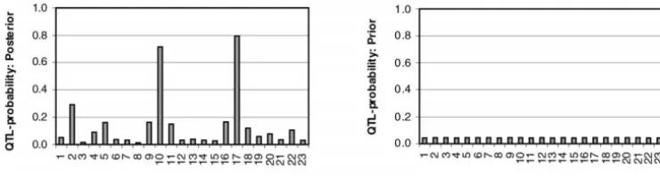
Figure 2.—QTL probabilities. Locus-specific estimates of QTL probabilities for the CF data set (left) and the corresponding prior probabilities (right) are shown. Marker numbers are shown on thex-axis and QTL probabilities on they-axis.
heritability of 0.63. Haldane’s function was used to con- corresponding QTL effect becomes negligible. In such case, a locus-indicator value is not sufficient alone to vert recombination fractions to morgans. The
in-termarker genetic distances are wide in this data set, determine how well the putative position explains the phenotype. However, we can still inspect their values as typically corresponding to recombination fractions of
0.1 or 0.2. The complete data set was used here (without preliminary indicators of QTL activity. In particular due to the relatively small amount of LD in the data set (see any missing values), whereasKilpikariandSillanpa¨a¨
(2003) used the data set where 20% of the marker geno- below) and the “shrinkage” assumption in our model, we obtained a clear indication of QTL positions at the types were missing. Unlike in CF and FA analyses, every
individual contributed a single observation (one pheno- probability scale. Figure 2 (left) shows a distinct signal at the correct ⌬F508 position on marker 17, which is type and two alleles at each locus) to the analysis where
a random-variance model, with for each allele its own known to account for ⵑ66% of the disease chromo-somes (BertranpetitandCalafell 1996). Addition-coefficient, was assumed.
Analyses: Data sets were analyzed in WinBUGS 1.3 ally a clear signal appears at marker 10 (EG1.4) outside the CFTR region. This location as well as many others
(Gilkset al.1994;Spiegelhalteret al.1999), using a
Pentium 4, 2.8 GHz. In CF and FA analyses, where we was found to have a strong secondary association in the study of Keremet al. (1989). Moreover,Molitor et al.
assumed a prior distribution for or prior
indepen-dence of locus indicators, we ran two MCMC chains (2003b) used a single-locus model and found a bimodal posterior distribution for gene location with both modes each of length 30,000 (13,500 in FA analyses with fixed
and 5500 in simulation analyses) with different initial within 0.03 cM of our best candidates. They also made an additional analysis where the left mode disappears values. First, 5000 (1000 and 4000) rounds were
dis-carded from each chain as “burn-in,” which resulted in in an analysis for which the only case haplotypes were those known to contain the⌬F508mutation. Our method 50,000 (25,000 and 3000) pooled MCMC samples in
total, respectively. We did not apply any “thinning” for clearly identifies marker 10 as a secondary contributor in this data set. Because of this, we performed a closer the chain, because of sufficient computer storage
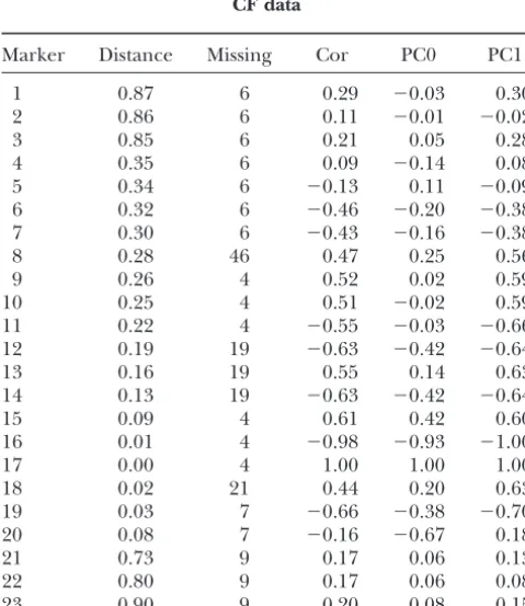
capac-ity and low autocorrelation in the samples. The two inspection of haplotypes in the original data set. In Table 1, one can see that occurrences of certain alleles MCMC chains were run in parallel, which tookⵑ20 hr
with CF data and 8 (4) hr with FA data (with fixed at markers 10 and 17 correlate with each other in haplo-types (correlation is 0.51). Moreover, one can say that ) and 98 hr with simulated data. The convergence
assessments were performed by visually monitoring correlation between markers 10 and 17 is surprisingly chains for several different parameters. low (⫺0.02) among control individuals (Table 1, PC0), suggesting that locus 10 may have protective influence (negative susceptibility) on the disease. A possible rea-RESULTS son why this locus has not been suggested by others is
that most LD mapping approaches focus on searching CF data:In Figure 2, we present the estimated
poste-for susceptibility alleles only. Note that although the rior probabilities for different markers to be associated
posterior estimated number of trait loci was three, Fig-on the CF phenotype (left) and the same based Fig-on prior
ure 2 clearly supported only two locations with several only (right). The posterior estimate for the number of
neighboring locations with much smaller QTL probabil-trait loci in the whole region turned out to beⵑ3 (with
ities. We believe that this estimated number reflects a mean 3.24 and mode 3) where the prior assumption
marker dependency (LD) pattern rather than the actual for the same was 1.
QTL number for the region (seediscussion). QTL probabilities in our model may be confounded
In Figure 3 (left), the posterior plot of estimated with QTL effects. This is because in the case of strong
allelic effects consistently supported the same two mark-LD (dependence), the prior of locus indicators supports
ers (10 and 17) as indicated in Figure 2. One can see several indicators to have value one simultaneously. At
large and opposite effects of two alleles at these markers. the same time, if the position with indicator value one
Figure3.—QTL allelic effects. Locus-specific point estimates (mean) of allelic effects for the CF data set (left) and the corre-sponding prior (right) are shown. The first and the second allele at each marker locus are shown as open and solid bars, respectively. These quantities are calculated on the basis of pooling samples from two separate MCMC chains with 30,000 samples (after an initial 5000 burn-in rounds) in each. All sampled values were utilized in these estimates, including the iterations where the marker indicator was zero. Marker numbers are shown on thex-axis and the underlying hidden phenotype (liability) scale is on they-axis. Note that the effects are double in size.
is comparable to the estimated effect obtained under practice and as mentioned before, estimates for the QTL positions and their effects may be confounded. the model where the first coefficient at each locus is
constrained to zero. For comparison, the right side of Therefore, a more robust way of analyzing association in such confounded models can be done by combining Figure 3 shows allelic effects under the prior model
(without data). Note that effect estimates shown in Fig- two sources of posterior information (QTL and their effects) into a single marker-specific summary that can ure 3 are point estimates (mean) whereas the whole
distribution is summarized for loci 10 and 17 in Table 2. be called a weighted genetic variance. This may be ob-tained from the posterior distribution of the product In general, effect estimation can be inaccurate in
of indicator variable Il and either absolute difference (biallelic case) or variance (multiallelic case) of allelic
TABLE 1 effects la’s at each location l. For biallelic loci, this
summary corresponds to a model-averaged effect
esti-CF data
mate (averaged over all models with the effect set to Marker Distance Missing Cor PC0 PC1 zero in models where the marker was not selected) proposed by Ball(2001) and a model-averaged
vari-1 0.87 6 0.29 ⫺0.03 0.30
ance estimate for multiallelic markers. However, for the
2 0.86 6 0.11 ⫺0.01 ⫺0.02
present analysis, this practice produced a picture similar
3 0.85 6 0.21 0.05 0.28
4 0.35 6 0.09 ⫺0.14 0.08 to Figure 2 (with an approximate scale difference). A 5 0.34 6 ⫺0.13 0.11 ⫺0.09 related approach of combining posterior information 6 0.32 6 ⫺0.46 ⫺0.20 ⫺0.38 on QTL and their effects using Bayesian QTL mapping 7 0.30 6 ⫺0.43 ⫺0.16 ⫺0.38 and variance component models has been proposed in
8 0.28 46 0.47 0.25 0.56
XuandYi(2000).
9 0.26 4 0.52 0.02 0.59
Linkage disequilibrium pattern due to close linkage
10 0.25 4 0.51 ⫺0.02 0.59
of loci: Instead of estimating LD as a degree of joint
11 0.22 4 ⫺0.55 ⫺0.03 ⫺0.66
12 0.19 19 ⫺0.63 ⫺0.42 ⫺0.64 occurrence of alleles at two loci (which requires haplo-13 0.16 19 0.55 0.14 0.63 type data), we assume that the effect of LD should also 14 0.13 19 ⫺0.63 ⫺0.42 ⫺0.64 be visible in the behavior of locus indicators (in the 15 0.09 4 0.61 0.42 0.60 case that they are not confounded; otherwise a weighted
16 0.01 4 ⫺0.98 ⫺0.93 ⫺1.00
genetic variance may be selected). We express the strength
17 0.00 4 1.00 1.00 1.00
18 0.02 21 0.44 0.20 0.63
19 0.03 7 ⫺0.66 ⫺0.38 ⫺0.70 TABLE 2
20 0.08 7 ⫺0.16 ⫺0.67 0.18
CF data
21 0.73 9 0.17 0.06 0.13
22 0.80 9 0.17 0.06 0.08
23 0.90 9 0.20 0.08 0.15 Marker Allele Mean SD 2.5% 97.5%
Marker, the distance (in centimorgans) of the marker from 10 1 0.62 0.89 ⫺1.35 2.20 locus 17; Missing, the number of missing alleles; Cor, pairwise 2 ⫺0.70 0.91 ⫺2.31 1.36 coefficient of phi-correlation (between the marker and locus 17 1 0.77 0.85 ⫺1.19 2.28 17); PC0, pairwise phi-correlation between the marker and 2 ⫺0.83 0.86 ⫺2.31 1.17 locus 17 for individuals with phenotype status zero; PC1,
pair-wise phi-correlation between the marker and locus 17 for Posterior estimates for gene effects (mean), the standard deviation of posterior distribution (SD), and 2.5 and 97.5% individuals with phenotype status one. The phi-correlation
coefficient, which is a variant of Pearson’s correlation coeffi- quantiles of the posterior distribution of the gene effects of the two alleles at candidate marker positions 10 and 17 are cient for binary variables (Yule1912), is calculated only from
Figure4.—Estimated linkage disequilib-rium pattern for the CF data set. The poste-rior probabilities of jointly selecting two ad-jacent markers into the model (i.e., their indicators have value one simultaneously) are estimated for each marker pair (dia-mond, scale in the right y-axis). For each marker pair, the corresponding prior (cir-cle, scale in the righty-axis) and the physical distance between markers are also shown (box, scale in the lefty-axis). Markers pres-ent in each marker pair are shown on the x-axis.
of LD as a probability of an event that two adjacent an estimated age of⌬F508 to be near 200 (Serre et al. 1990;Morriset al.2000). However, recall that our esti-markers have value one simultaneously in their locus
indicators (this event is called joint selection). Figure 4 mate is averaged over all trait loci (positions 10 and 17) and does not represent only the CFTR region. There-shows distinctly elevated posterior probabilities of joint
selection around marker 17 and also around marker 10 fore, we did yet another analysis and allowed two age parameters, one for the CFTR region (markers 16–20) (although not so high) compared to prior levels of LD.
Inference about estimated average age of mutations and another outside of it (models not shown). The new analysis resulted in posterior means of the two age over trait loci:Sometimes it may not be simple to
param-eterize the model to obtain a direct posterior of a certain parameters to be 207 (with 95% credible interval [205, 208]) at the CFTR region and 319 (with 95% credible quantity of interest analytically, as is the case here. To
make inference about such a stochastic function of the interval [316, 321]) elsewhere (i.e., dominated by posi-tion 10). This result is also in agreement with the idea posterior distribution, a sequential analysis can be
car-ried out by using posterior samples generated by a first that position 10 may have protective influence because it is very likely that mutations with protective effects are Bayesian analysis as data in a second Bayesian analysis.
We performed such an additional analysis for a posterior older than others.
Sensitivity analyses: To study sensitivity of the esti-sample of locus indicators to estimate the average age
of mutations over trait loci. In this second Bayesian mates of age of mutationa, we performed test trials assum-ing Gamma(5, 0.05), Gamma(1, 1), or Gamma(10, 0.1) analysis, 30,000 MCMC samples were considered as
ac-tual data points consisting of sampled values of indica- prior fora. All priors led to the same posterior estimates, strongly supporting the estimated value.
torsxl⫽1{Il⫽Il⫺1⫽1}for each consecutive marker pair (l⫺
1,l) among 23 markers. In our model we assumed that The estimated posterior mean for the smoothing pa-rameterwas 100, corresponding closely to the prior indicators xl are Bernoulli distributed with parameter
e⫺adl, where a represents the average age of mutation mean. To check validity of this estimate we also used some other values for prior mean. These extra analyses over trait loci with a possible scale difference anddlis
the distance between consecutive markers of marker resulted in the posterior means of smoothing parameter values, which corresponded strongly to the prior as-pair (l⫺1,l). We assumed a Gamma(5, 0.05) prior for
age parameteraand ran two parallel chains with 3500 sumption, indicating that this quantity is very dependent on the prior choice. However, the posterior distribu-MCMC rounds (with 1000 burn-ins in each) resulting
altogether in 5000 pooled MCMC samples to be utilized tions of other parameters were not affected by the changes made to the prior for the smoothing parameter. for estimation. The sampler seemed to have converged
quickly. Note that although this model appears to be With CF data, we tested four different priors for allelic coefficients:N(0, 1),N(0, 10),N(0, 20), andN(0, 100). similar to the one used for smoothing, the smoothing
parameterdoes not have this interpretation because The change of prior had the largest influence on the convergence time but also increased variability at the it represents prior rather than posterior dependency
(linkage disequilibrium) along a chromosomal seg- mean level of posterior estimated allelic coefficients with increased variability (“flatness”) in the prior. Maxi-ment.
In the analysis described above, the estimated poste- mally a 2.5-fold change was observed in the estimated allelic coefficient by changing the prior. The influence rior mean of age a was 0.2679. Because 1 cM is ⵑ1
Mb in humans and our analyses were performed in was negligible to the absolute difference between coef-ficients. However, the same positions were supported kilobases, we have to multiply our estimate by 1000,
Figure5.—Locus-specific point estimates (mean) of weighted genetic variances for the Friedreich ataxia data. Different types of specifications for smoothing parameterare shown: (A) wide Gamma(1, 0.01) prior forwith mean 100 (posterior mean 62.65); (B) narrow Gamma(100, 1) prior forwith mean 100 (posterior mean 99.32); (C) ⫽10 (strong smoothing); (D) ⫽ 250 (weak smoothing); and (E) independent prior for indicators with no parameter (no smoothing). Marker numbers are shown on thex-axis and weighted genetic variances are on they-axis. Note that the variance parameter is for the model where the effects are double in size.
Friedrich ataxia data:Unlike with CF data, locus-indi- can see the posterior mean weighted genetic variance estimated at different marker positions. Two putative cator variables turned out to be confounded with QTL
effects in the Friedreich ataxia data (due to high LD). QTL positions at markers 3 and 5 are clearly indicated. It is known that the gene is located between markers 5 Therefore, we present posterior information on locus
indicators and effect parameters in a combined form and 6 (Liu et al. 2001). Note that the best putative candidate ofMolitoret al.(2003a) was marker 3. Again (weighted genetic variance). This quantity was calculated
at haplotypes of loci 3 and 5 among disease haplotypes indicators (that are created by transformation) can then be used as data for estimating age of mutation over trait (32/58 with haplotype 8-5 and 12/58 with haplotype
8-6) and to some extent also among control haplotypes loci or number of QTL similar to our CF analysis. To understand the transformation, let us first con-(11/69 with haplotype 8-5 and 3/69 with haplotype 8-6;
all results not shown). Joint occurrence among controls sider the marker-specific posterior for the weighted ge-netic variance. Note that only a single value (mean) of this is not conclusive due to a high number of missing alleles
at marker 5 (23/69). Simple odds ratio calculation for posterior is plotted at each marker point in Figure 5. Although the histogram estimates indicate these vari-alleles indicates enrichment of vari-alleles 3 and 5 of marker
5 and allele 8 of marker 3 among the cases with values ables to be stochastically ordered (for the FA data), in the absence of analytical forms (for these posteriors), 2.1, 2.3, and 2.5, respectively. However, allele 5 of
marker 5 occurs together in haplotypes with allele 8 we utilize only the tail-ordering property of the posteri-ors. For each marker, we estimated the corresponding of marker 3. The same was further supported by the
posterior estimates of individual allelic effects (results tail probability of exceeding the predefined percentile of the joint distribution of all weighted genetic variances. not shown). To conclude, most of the alleles that were
estimated to be enriched among cases occurred jointly [Alternatively, the cutoff point can be visually defined from the weighted genetic variance plot (Figure 5).] with a high frequency with either allele 3 of marker 5
or allele 8 of marker 3 (which also implies they occurred Mathematically this is a simple Bernoulli discretization of a continuous variable where the corresponding Ber-with alleles 5 or 6 of marker 5). Therefore all the
en-riched alleles of all markers could be approximately noulli probability then represents the probability for a marker to have a high or extreme value of the weighted represented by these two alleles at these two markers
together. This further supports two putative findings of genetic variance. These tail probabilities should be simi-lar in pattern (over markers) with those obtained by this analysis.
Figure 5 represents weighted genetic variance under the means as in Figure 5. (Assuming the means to be reasonable estimates of the central tendency of the different prior specifications for overall smoothing
pa-rameterand for locus indicators (each corresponding weighted genetic variances).
Estimated average age of mutations over trait loci and to a different level of smoothing). In Figure 5A one can
see that if we assume a wide prior for the smoothing their number in FA data:We performed several trials with different cutoff points put on the weighted genetic parameter, similarly as in the CF data, we obtain a
mod-erately smoothed posterior. In contrast, if a narrow prior variance and each time ran the separate age estimation analysis with MCMC using adjusted locus indicators as is given for the smoothing parameter (Figure 5B), we
obtain a posterior where the smoothing has become a data, as in CF analysis (results not shown). As expected, the estimated age depends on the stringency of the bit stronger (this is more visible in the estimated LD
pattern, results not shown). By comparing Figure 5E criteria used to define adjusted locus indicators. The higher the cutoff is put on the weighted genetic variance (no smoothing), Figure 5D (weak constant smoothing),
and Figure 5C (strong constant smoothing), one can the rarer the event becomes and the estimated age would increase accordingly. However, even with the choice of clearly see that signals at positions 3 and 5 become
stronger as levels of smoothing increase. Figure 5E cor- cutoff as 90th, 95th, and 99th percentiles (of the overall distribution) the posterior (median) age estimates were responds to the model, wherea prioriindependence of
locus indicators was assumed [cf.the model ofKilpikari 30, 42, and 66 generations (with narrow credible inter-vals), indicating this to be a recent mutation compared
andSillanpa¨a¨(2003), where all unoccupied QTL
posi-tions were considered to be equally likely]. to many others. The corresponding three estimates for the number of QTL were 1.2, 0.6, and 0.1, respectively. Dichotomizing transformation for weighted genetic
variance:Direct inference about estimated average age Three percentiles correspond to points 7.85, 13.29, and 33.65, respectively, in the weighted genetic variance of mutations over trait loci or number of QTL, as was
done for CF data, is not possible from FA data because scale (recall that only means are shown in Figure 5). On the basis of these trials, it seems that this practice the estimates of locus indicators and effects are
con-founded in the FA data due to high linkage disequilib- can provide useful information on the neighborhood of the age estimate rather than a unique estimate in rium. In other words, posterior weighted genetic
vari-ances clearly differ from posterior QTL probabilities. such cases where direct estimation is impossible due to confounding. However, this practice is not very suitable To estimate age of mutation (or number of QTL) under
this condition, we transform each (continuous) weighted for estimating the number of QTL.
Comparison of missing value imputation methods: genetic variance to a binary form that can be called an
adjusted locus indicator, which can then be collected On the basis of our numerical experiments with these data sets, it was clear that missing data imputation that together and plotted as QTL probabilities. The
QTL-probability plot drawn from adjusted indicators should was applied to the FA data (with the prior where each allele was considered as equally likely) was better be-resemble the plot drawn from weighted genetic variances
Figure6.—Locus-specific estimates of QTL probabilities (left) and weighted genetic vari-ances (right) for the simulated data set, where loci 18 and 22 represent the true gene loca-tions. Marker numbers are shown on the x-axis and QTL probabilities/weighted ge-netic variances are on they-axis.
for allele frequency hyperparameters), providing faster effects) into the phenotype model is straightforward in WinBUGS. However, the overall smoothing parameter convergence.
Simulated data: As expected, in large genomic re- can be thought of as a special tuning parameter in our model, which should not be too small in data sets gions this model seems to behave in a closely similar
fashion to the model ofKilpikariandSillanpa¨a¨(2003). with strong LD. With small values, the dependence be-tween adjacent locus indicators may become too strong, In Figure 6 (left), one can see that the posterior QTL
probability is practically zero at most of the markers practically preventing the MCMC sampler from moving (insufficient mixing). This may also happen with some (except some faint pattern due to LD) while it is one
at true QTL locations (18 and 22). Recall that marker prior distributions, which allow small values for . Therefore, one should be careful when analyzing data 25 showed a weak signal in Kilpikari andSillanpa¨a¨
(2003), which we think is due to missing values in the sets known to have strong LD.
We share the view ofPhillipset al.(2003) andMorris
analyzed data set. The same two positions (18 and 22)
are supported also in Figure 6 (right), which presents et al.(2003b) that the block structure of LD in the human genome creates a need for sophisticated modeling to weighted genetic variances for the data. Note that it is
clearly visible that position 18 had a stronger effect than refine locations within the LD blocks. (For the opposite view, see Goldstein2001.) ContiandWitte (2003) 22. The posterior (mean) estimate for the number of QTL
in the whole region was 2. Closer inspection of locus demonstrated how haplotype block information (Daly
et al.2001;Goldstein2001;Gabrielet al.2002;Wall
indicators showed that some dependence between
indica-tors was found only between markers 15–16 and 31–34, and Pritchard 2003) can be easily incorporated in their model so that marker-specific gene effects “bor-where the intermarker distances were the smallest
(recom-bination fractions for the two regions were 0.02 and [0.02, rowed information” or were depending on each other only within the same block. The same goal (indepen-0.01, 0.01], respectively; results not shown).
dence of markers between blocks) can be obtained in our model by artificially replacing the known distance DISCUSSION
between block-boundary markers (adjacent markers that are members in different blocks) with some arbitrarily We have presented a new multilocus method for
asso-ciation mapping in short chromosomal intervals, where large value corresponding to independence of loci. Uti-lization of block information corresponds to accounting covariances between markers are accounted for by using
available physical or genetic distance information. Ac- for common population ancestry (LD due to covariance between haplotypes).
counting for these covariances corresponds to spatial
smoothing of association signals (LD measured from locus Population stratification is a well-known problem with association studies (Cardon and Palmer 2003). The indicators) along the candidate region. The method is
suitable for genotype data on multiallelic markers and benefit of the “LD smoothing” approach presented here is that it can control fluctuations in LD (spurious associa-is equally applicable for quantitative and binary traits
and can handle some degree of missing observations. tions) due to several factors including events in population history. This way one does not need to apply matching One can also estimate the age of the variant, which
should be interpreted here as time to the most recent (Hindet al.2004) or utilize techniques such as genomic controls (DevlinandRoeder1999) or structured associa-common ancestor rather than to actual age of mutation,
which can be much older (RannalaandSlatkin1998). tion (Pritchard et al.2000a,b; Sillanpa¨a¨ et al.2001;
Coranderet al.2003, 2004;Hoggartet al.2003), which
One advantage of this method is that it can be
imple-mented with WinBUGS (see Congdon 2001), which use an external set of unlinked markers. If the sample consists of related individuals with known relationships, avoids user specification of data-specific tuning
parame-ters needed in the Metropolis-Hastings random-walk inclusion of a polygenic component into the association model could take away a stratification problem completely algorithm (ChibandGreenberg1995). Moreover,
els that combine pedigree and linkage disequilibrium in- ingful to estimate the number of QTL as the number of trait-associated marker segments rather than as the formation (Meuwissenet al.2002;Perez-Enciso2003;
number of individual trait-associated markers (see Ter-FanandJung 2003;Lundet al.2003;Meuwissenand
willigeret al.1997;ChapmanandThompson2002).
Goddard2004).
The alternative, illustrated with FA data, to estimate the The postgenomic era is bringing us a vast amount
number of QTL from transformed data, did not seem of external public information on the human genome
to perform well. One potential future approach to re-sequence.RannalaandReeve(2001) proposed
utiliza-duce or better control confounding in our model would tion of such information by specifying an informative
be to apply stochastic search variable selection (SSVS; prior distribution for the location of a disease gene in
GeorgeandMcCulloch1993;Yiet al.2003;
Meuwis-their Bayesian LD analysis. An informative prior
provid-sen and Goddard 2004) so that locus indicators are
ing information on gene-rich areas or distribution of
hierarchically controlling the prior of QTL effects. A exons and introns in the candidate region will improve
well-known drawback in SSVS is that it requires addi-gene localization. To utilize this type of external
infor-tional tuning parameters (pseudo-priors), which are mation in our model, one can modify the prior for
data dependent (Dellaportaset al.2000). In any case, locus-specific indicatorsp(Il|Il⫺1,s, ,dl) by specifying
the subset selection of candidate markers should be individual values of shrinkage factor 1⫺sat each locus,
done by the analyst on the basis of the highly elevated reflecting the prior probability of the position
(locus-locus-specific QTL probabilities or weighted genetic specific sl should then be scaled so that they sum up
variances in contrast to selection based on markers show-to the prior number of QTL in regionR).
ing smallP-values in classical association testing. By do-We want to briefly comment on our choice of a
logit-ing so a Bayesian analysis avoids complicated problems link function here in contrast to a probit link that was
in multiple testing. On the other hand, Bayesian analysis used inKilpikariandSillanpa¨a¨(2003). The logit link
requires attention to monitoring of convergence and was chosen here because of its good mixing properties
inspection of mixing properties of the MCMC sampler. in WinBUGS (A. Thomas, personal communication).
Also so-called sensitivity analysis is an important part of Additionally, although probit and logit-link functions
good analysis practice. are very close to each other, only logit link is robust
We have put the model specification code (written in for ascertainment (Kagan2001; Neuhaus2002). The
the BUGS language) at URL: http://www.rni.helsinki.fi/ choice of probit link, implemented via data
augmen-ⵑmjs/. This code is freely available for research purposes. tation, was motivated inKilpikariandSillanpa¨a¨(2003)
by the technical fact that one was able to apply exactly We are grateful to Jules Herna´ndez-Sa´nchez and Andrew Thomas for helpful discussions and two anonymous reviewers for comments
the same MCMC sampler (including the full
condition-that greatly improved the presentation of the results. This work was
als) for all underlying model parameters in both
quanti-supported by a research grant (202324) from the Academy of Finland
tative and binary traits. and by the Centre of Population Genetic Analyses, University of Oulu, In some cases, the number of QTL-effect parameters Finland.
(categories) considered in the model may become too large to model each parameter with a fixed-variance model (fixed-effect model). Such a situation may arise
LITERATURE CITED if the number of distinct alleles segregating in a marker
Ball, R. D., 2001 Bayesian methods for quantitative trait loci
map-is very high or one considers gene-gene or
gene-environ-ping based on model selection: approximate analysis using
Bayes-ment interactions or genotype/haplotype-specific ef- ian information criterion. Genetics159:1351–1364.
fects in the phenotype model. In an alternative to the Bertranpetit, J., andF. Calafell, 1996 Genetic and geographical variability in cystic fibrosis: evolutionary considerations, pp. 97–
random-variance model (“variance component model”),
114 inVariation in the Human Genome, edited by D.Chadwick
which avoids these problems, one can coarse the num- and G.Cardew. Wiley, Chichester, England.
ber of groups by regrouping alleles or genotypes/haplo- Broman, K. W, andT. P. Speed, 2002 A model selection approach for identification of quantitative trait loci in experimental crosses.
types into a small number of new groups on the basis
J. R. Stat. Soc. B64:641–656.
of some simple rule. A more sophisticated solution is Cardon, L. R., andL. J. Palmer, 2003 Population stratification and to include partitioning as a part of the model following spurious allelic association. Lancet361:598–604.
Chapman, N. H., andE. A. Thompson, 2002 The effect of
popula-ideas inSeamanet al.(2002).
tion history on the length of ancestral segments. Genetics162:
Estimates for the number of QTL in studies, which 449–458.
concentrate on small chromosomal intervals, are con- Chib, S., andE. Greenberg, 1995 Understanding the Metropolis-Hastings algorithm. Am. Stat.49:327–335.
founded by strong LD (dependence) between markers.
Clayton, D., 2000 Linkage disequilibrium mapping of disease
sus-It is very likely that more than just a single marker is in ceptibility genes in human populations. Int. Stat. Rev.68:23–43. strong LD with the true QTL and therefore they show Congdon, P., 2001 Bayesian Statistical Modelling. John Wiley & Sons,
Chichester, UK.
elevated gene activity, as illustrated in CF and FA data.
Conti, D. V., andJ. S. Witte, 2003 Hierarchical modeling of linkage
Because LD appears as continuous segments around disequilibrium: genetic structure and spatial relations. Am. J.
Hum. Genet.72:351–363.
mean-Conti, D. V., V. Cortessis, J. Molitor andD. C. Thomas, 2003 librium by the decay of haplotype sharing, with application to fine scale genetic mapping. Am. J. Hum. Genet.65:858–875. Bayesian modeling of complex metabolic pathways. Hum. Hered.
56:83–93. Meuwissen, T. H. E., andM. E. Goddard, 2000 Fine mapping of quantitative trait loci using linkage disequilibrium with closely
Corander, J., P. WaldmannandM. J. Sillanpa¨a¨, 2003 Bayesian
analysis of genetic differentiation between populations. Genetics linked marker loci. Genetics155:421–430.
Meuwissen, T. H. E., andM. E. Goddard, 2004 Mapping multiple
163:367–374.
Corander, J., P. Waldmann, P. MarttinenandM. J. Sillanpa¨a¨, QTL using linkage disequilibrium and linkage analysis informa-tion and multitrait data. Genet. Sel. Evol.36:261–279. 2004 BAPS 2: enhanced possibilities for the analysis of the
ge-netic population structure. Bioinformatics20:2363–2369. Meuwissen, T. H. E., B. J. HayesandM. E. Goddard, 2001 Predic-tion of total genetic value using genome-wise dense marker maps.
Cordell, H. J., andR. C. Elston, 1999 Fieller’s theorem and linkage
disequilibrium mapping. Genet. Epidemiol.17:237–252. Genetics157:1819–1829.
Meuwissen, T. H. E., A. Karlsen, S. Lien, I. OlsakerandM. E. Daly, M. J., J. D. Rioux, S. F. Schaffer, T. J. HudsonandE. S.
Lander, 2001 High-resolution haplotype structure in the hu- Goddard, 2002 Fine mapping of a quantitative trait locus for twinning rate using combined linkage and linkage disequilibrium man genome. Nat. Genet.29:229–232.
Dellaportas, P., J. J. ForsterandI. Ntzoufras, 2000 Bayesian mapping. Genetics161:373–379.
Molitor, J., P. MarjoramandD. Thomas, 2003a Fine-scale map-variable selection using the Gibbs sampler, pp. 273–286 in
General-ized Linear Models: A Bayesian Perspective, edited by D. K.Dey, S. K. ping of disease genes with multiple mutations via spatial clustering techniques. Am. J. Hum. Genet.73:1368–1384.
Ghoshand B. K.Mallick. Marcel Dekker, New York.
Devlin, B., andK. Roeder, 1999 Genomic control for association Molitor, J., P. MarjoramandD. Thomas, 2003b Application of Bayesian spatial statistical methods to analysis of haplotypes ef-studies. Biometrics55:997–1004.
Devlin, B., K. RoederandL. Wasserman, 2003 Analysis of multilo- fects and gene mapping. Genet. Epidemiol.25:95–105.
Morris, A., J. C. WhittakerandD. J. Balding, 2000 Bayesian fine-cus models of association. Genet. Epidemiol.25:36–47.
Durrant, C., K. T. Zondervan, L. R. Cardon, S. Hunt, P. Deloukas scale mapping of disease loci, by hidden Markov models. Am. J. Hum. Genet.67:155–169.
et al., 2004 Linkage disequilibrium mapping via cladistic analysis
of single-nucleotide polymorphism haplotypes. Am. J. Hum. Morris, A., A. PedderandK. Ayres, 2003a Linkage disequilibrium assessment via log-linear modeling of SNP haplotype frequencies. Genet.75:35–43.
Fan, R., andJ. Jung, 2003 High-resolution joint linkage disequilib- Genet. Epidemiol.25:106–114.
Morris, A. P., J. C. Whittaker, C.-F. Xu, L. K. HostingandD. J.
rium and linkage mapping of quantitative trait loci based on
sibship data. Hum. Hered.56:166–187. Balding, 2003b Multipoint linkage-disequilibrium mapping narrows location interval and identifies mutation heterogeneity.
Flint, J., andR. Mott, 2001 Finding the molecular basis of
quantita-tive traits: successes and pitfalls. Nat. Rev. Genet.2:437–445. Proc. Natl. Acad. Sci. USA100:13442–13446.
Morton, N. E., W. Zhang, P. Taillon-Miller, S. Ennis, P.-Y. Kwok Gabriel, S. B., S. F. Schaffer, H. Nguyen, J. M. Moore, J. Royet al.,
2002 The structure of haplotype blocks in the human genome. et al., 2001 The optimal measure of allelic association. Proc. Natl. Acad. Sci. USA98:5217–5221.
Science296:2225–2229.
George, E. I., andR. E. McCulloch, 1993 Variable selection via Neuhaus, J. M., 2002 Bias due to ignoring the sample design in case-control studies. Aust. N. Z. J. Stat.44:285–293.
Gibbs sampling. J. Am. Stat. Assoc.88:881–889.
Gilks, W. R., A. ThomasandD. J. Spiegelhalter, 1994 A language Nordborg, M., andS. Tavare, 2002 Linkage disequilibrium: what history has to tell us. Trends Genet.18:83–90.
and program for complex Bayesian modeling. Statistician 43:
169–178. Perez-Enciso, M., 2003 Fine mapping of complex trait genes com-bining pedigree and linkage disequilibrium information: a
Bayes-Goldstein, D. B., 2001 Islands of linkage disequilibrium. Nat.
Genet.29:109–111. ian unified framework. Genetics163:1497–1510.
Phillips, M. S., R. Lawrence, R. Sachidanandam, A. P. Morris, Greenland, S., J. A. SchwartzbaumandJ. A. Finke, 2000 Problems
due to small samples and sparse data in conditional logistic regres- D. J. Baldinget al., 2003 Chromosome-wide distribution of haplotype blocks and the role of recombination hot spots. Nat. sion analysis. Am. J. Epidemiol.151:531–539.
Hind, D. A., R. P. Stokowski, N. Patil, K. Konvicka, D. Kersheno- Genet.33:382–387.
Piepho, H.-P., and H. G. Gauch, Jr., 2001 Marker pair selection
bich et al., 2004 Matching strategies for genetic association
studies in structured populations. Am. J. Hum. Genet.74:317– for mapping quantitative trait loci. Genetics157:433–444.
Pritchard, J. K., M. StephensandP. Donnelly, 2000a Inference 325.
Hoggart, C. J., E. J. Parra, M. D. Shriver, C. Bonilla, R. A. Kittles of population structure using multilocus genotype data. Genetics
155:945–959.
et al., 2003 Control of confounding in genetic associations in
stratified populations. Am. J. Hum. Genet.72:1492–1504. Pritchard, J. K., M. Stephens, N. A. RosenbergandP. Donnelly, 2000b Association mapping in structured populations. Am. J.
Kagan, A., 2001 A note on the logistic link function. Biometrika
88:599–601. Hum. Genet.67:170–181.
Rannala, B., andJ. P. Reeve, 2001 High-resolution multipoint
link-Kerem, B.-S., J. M. Rommens, J. A. Buchanan, D. Markiewicz, T. K.
Coxet al., 1989 Identification of the cystic fibrosis gene: genetic age-disequilibrium mapping in the context of a human genome sequence. Am. J. Hum. Genet.69:159–178.
analysis. Science245:1073–1080.
Kilpikari, R., andM. J. Sillanpa¨a¨, 2003 Bayesian analysis of multilo- Rannala, B., andM. Slatkin, 1998 Likelihood analysis of disequilib-rium mapping, and related problems. Am. J. Hum. Genet.62:
cus association in quantitative and qualitative traits. Genet.
Epide-miol.25:122–135. 459–473.
Risch, N., andK. Merikangas, 1996 The future of genetic studies
Kuo, L., andB. Mallick, 1998 Variable selection for regression
models. Sankhya Ser. B60:65–81. of complex human diseases. Science273:1616–1617.
Sasieni, P. D., 1997 From genotypes to genes: doubling the sample
Lazzeroni, L. C., 1998 Linkage disequilibrium and gene mapping:
an empirical least-squares approach. Am. J. Hum. Genet. 62: size. Biometrics53:1253–1261.
Seaman, S. R., S.Richardson, I.Stu¨ ckerand S.Benhamou, 2002 159–170.
Lazzeroni, L. C., 2001 A chronology of fine-scale gene mapping A Bayesian partition model for case-control studies on highly polymorphic candidate genes. Genet. Epidemiol.22:356–368. by linkage disequilibrium. Stat. Methods Med. Res.10:57–76.
Liu, J. S., C. Sabatti, J. Teng, B. J. B. KeatsandN. Risch, 2001 Sen, S., andG. A. Churchill, 2001 A statistical framework for quan-titative trait mapping. Genetics159:371–387.
Bayesian analysis of haplotypes for linkage disequilibrium
map-ping. Genome Res.11:1716–1724. Serre, J. L., B. Simon-Bouy, E. Morret, B. Jaume-Roig, A. Balasso
-poulouet al., 1990 Studies of RFLPs closely linked to the
cystic-Lund, M. S., P. Sorensen, B. GuldbrandtsenandD. A. Sorensen,
2003 Multitrait fine mapping of quantitative trait loci using fibrosis locus throughout Europe lead to new consideration in population genetics. Hum. Genet.84:449–454.
combined linkage disequilibria and linkage analysis. Genetics
163:405–410. Service, S. K., D. W. Lang, N. B. FreimerandL. A. Sandkuijl, 1999 Linkage-disequilibrium mapping of disease genes by
disequi-tion of ancestral haplotypes in founder populadisequi-tions. Am. J. Hum. trait loci using Bayesian analysis and Markov chain Monte Carlo algorithms. Genetics146:735–743.
Genet.64:1728–1738.
Sillanpa¨a¨, M. J., andE. Arjas, 1998 Bayesian mapping of multiple Uimari, P., andM. J. Sillanpa¨a¨, 2001 Bayesian oligogenic analysis of quantitative and qualitative traits in general pedigrees. Genet. quantitative trait loci from incomplete inbred line cross data.
Genetics148:1373–1388. Epidemiol.21:224–242.
Wall, J. D., andJ. K. Pritchard, 2003 Haplotype blocks and linkage
Sillanpa¨a¨, M. J., R. Kilpikari, S. Ripatti, P. OnkamoandP. Uimari,
2001 Bayesian association mapping for quantitative traits in a disequilibrium in the human genome. Nat. Rev. Genet.4:587– 597.
mixture of two populations. Genet. Epidemiol. 21(Suppl. 1):
S692–S699. Xu, S., 2003 Estimating polygenic effects using markers of the entire genome. Genetics163:789–801.
Spiegelhalter, D. J., A. ThomasandN. G. Best, 1999 WinBUGS
Version 1.2 User Manual. MRC Biostatistics Unit, Cambridge, UK. Xu, S., andN. Yi, 2000 Mixed model analysis of quantitative trait
Tanksley, S. D., 1993 Mapping polygenes. Annu. Rev. Genet.27: loci. Proc. Natl. Acad. Sci. USA97:14542–14547.
205–233. Yi, N., 2004 A unified Markov chain Monte Carlo framework for
Terwilliger, J. D., W. D. Shannon, G. M. Lanthrop, J. P. Nolan, mapping multiple quantitative trait loci. Genetics167:967–975.
L. R. Goldinet al., 1997 True and positive peaks in genomewide Yi, N., V. GeorgeandD. B. Allison, 2003 Stochastic search variable scans: applications of length-biased sampling to linkage mapping. selection for identifying multiple quantitative trait loci. Genetics Am. J. Hum. Genet.61:430–438. 164:1129–1138.
Thomas, D., D. O. Stram, D. Conti, J. MolitorandP. Marjoram, Yule, G. U., 1912 On the methods of measuring association between 2003 Bayesian spatial modeling of haplotype association. Hum. two attributes. J. R. Stat. Soc.75:576–642.
Hered.56:32–40.