Article
An Introduction to the Non-Equilibrium Steady
States of Maximum Entropy Spike Trains
Rodrigo Cofré1, Leonardo Videla1, Fernando Rosas2,3,4
1 CIMFAV, Facultad de Ingeniería, Universidad de Valparaíso, Valparaíso, Chile;
[email protected],[email protected]
2 Centre for Psychedelic Research, Department of Medicine, Imperial College London, London, UK;
3 Centre for Complexity Science and Department of Mathematics, Imperial College London, London, UK 4 Data Science Institute, Imperial College London, London, UK
1
2
3
4
5
6
7
8
* Correspondence:[email protected]
Abstract: Althoughmostbiologicalprocessesarecharacterizedbyastrongtemporalasymmetry, several popular mathematical models neglect this issue. Maximum entropy methods provide aprincipled wayof addressing time irreversibility, whichleveragespowerful results andideas fromthe3literatureofnon-equilibriumstatisticalmechanics. Thisarticleprovidesacomprehensive overviewof theseissues, withafocusinthe caseofspiketrainstatistics. Weprovideadetailed accountofthe5mathematicalfoundationsandworkoutexamplestoillustratethekeyconceptsand resultsfromnon-equilibriumstatisticalmechanics.
Keywords: non-equilibriumsteadystates;maximumentropyprinciple;spiketrainstatistics;entropy production
9
1. Introduction 10
Being the brain one of the most complex system within the observable universe, it is not surprising 11
that there is still a large number of unanswered questions related to its structure and functions. With 12
the aim of developing new ways of addressing such questions, there is an increasing consensus among 13
neuroscientists in that interdisciplinary approaches are promising. As a prominent example of this, 14
computational neuroscience have been greatly enriched during the last decades by tools, ideas and 15
methods coming from statistical physics [1,2]. Moreover, these methods are recently being revisited 16
with renewed interest due to the arrival of experimental techniques that generate huge volumes of 17
data. In particular, neuroscientists have become progressively aware of the powerful computational 18
techniques used by statistical physicist to analyze experimental data and large scale simulations. 19
When studying the firing patterns of collections of neurons, one of the most popular methods 20
from statistical mechanics is themaximum entropy principle(MEP), which builds the least structured 21
model that is consistent with average values measured from experimental data. These average values 22
are usually restricted to firing rates and synchronous pairwise correlations, which gives rise to models 23
composed by time independent and identically distributed (i.i.d) random variables, i.e. stochastic 24
processes without temporal structure [3–5]. Needless to say, there exists strong evidence in favour of 25
memory effects playing a major role in spike train statistics, and biological process in general [6–9]. 26
Following this evidence, over the last years the study of complex biological systems has started to 27
consider time-dependent processes where the past have an influence on future behavior [10–12]. The 28
corresponding asymmetry between past and future is called the “arrow of time”, which is the unique 29
direction associated with the irreversible flow of time that is noticeable in most biological systems. 30
Interestingly, the statistical physics literature has a fertile toolkit for studying time asymmetric 31
processes [13]. First, one introduces the distinction between steady states that imply thermal 32
equilibrium, and steady states that still carry fluxes – being called non-equilibrium steady states 33
(NESS). Additionally, the extend to which a steady-state is not in equilibrium (i.e. the strength 34
of it associated currents) can be quantified by theentropy-production rate[14], which is associated 35
with the degree of time-irreversibility in the corresponding process [14]. Theoretical studies have 36
recognized that being out-of-equilibrium is one of the distinctive properties of living systems [15–17]. 37
Consequently, any statistical description that is consistent with the out-of-equilibrium condition of 38
living neuronal networks should reflect some degree of time asymmetry, which can be characterized 39
using Markov chains [11,18–22]. 40
Despite of the potential of interdisciplinary pollination in these fascinating issues, many scientists 41
find hard to explore these possibilities because for the major entry barriers, which include differences 42
in jargon, conventions, and notations across the various fields. With this in mind, and with the aim to 43
foster the collaboration among disciplines, this article provides an introduction to these topics suitable 44
for researchers in the fields of physics or mathematics who are curious about the interesting questions 45
and possibilities that computational neurosciences offers. The focus on this community is motivated 46
by the growing community of mathematical physicists interested in computational neroscience. 47
The rest of this article is structured as follows. First, Section2introduce basic concepts of neural 48
spike trains and Markov processes. Then, Section3introduces the notion of observable, and explore 49
their fundamental properties. Section4then introduces the core ideas of MEP, proposing the formal 50
question and exploring methods for solving it. Section5studies various properties of interest of MEP 51
models, including fluction-dissipation relationships, and their entropy production. Finally, Section6 52
summarizes our conclusions. 53
2. Preliminary considerations 54
This section introduces definitions, notations, and conventions that are used throughout the 55
article in order to provide the necessary background to the unfamiliar reader. 56
2.1. Binning and spike trains 57
Consider a network ofNspiking neurons, where time has been binned (i.e. discretized) in such a 58
way that each neuron can exhibit no more than one action potential within one time bin∆tb. Action 59
potentials, or “spikes”, are “all-or-none” events, and hence spike data can be encoded using sequences 60
of zeros and ones. A spiking state is denoted byxkt =1, and correspond to the event in which thek-th 61
neuron spikes during thet-th time bin, whilextk=0 implies that it remains silent. 62
Aspike patterncorresponds to the spike-state of all neurons at time bint, denoted byxt:=xkt
N
k=1.
63
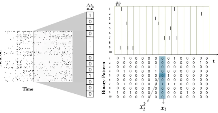
Aspike blockis a consecutive sequence of spike patterns, denoted byxt,r :=xsrs=t(see figure1). While 64
the length of the spike blockxt,r isr−t+1, is also useful to consider spike blocks of infinite length 65
starting from timet=0, which are denoted byx. Finally, in this work we consider that aspike trainis 66
an infinite sequence of spiking patterns. This assumption turn out to be useful because it allows to put 67
our analysis in the framework of stochastic processes, and because it allows to characterize asymptotic 68
statistical properties. 69
The set of all possible spike patters (or state space) corresponding to a network ofNneurons is 70
denoted byS, and the set of possible spike blocks of lengthRcorresponding to a network ofNneurons 71
Figure 1.Illustration of a spike train, a spiking state and spike pattern. The time bin size∆tbdetermine the binary patterns.
2.2. Elementary properties of Markov chains 73
A stochastic process is a collection of random variablesXt ∈ Sindexed byt ∈ T that often 74
refers to time. The setSrepresents the phase-space of the process; in the case of stochastic processes 75
representing spike trains, one usually takesS={0, 1}N. Moreover, considering the temporal binning 76
discussed in Section2.1, usuallyT=N, corresponding to the so-called discrete-parameter stochastic 77
processes. 78
While spike trains can be characterized by stochastic processes dependent on an infinite past (non-Markovian) in mathematical models [23,24], Markov chains are particularly well-suited for modeling data sequences with not-too-strong temporal dependencies. A stochastic process(Xt:t∈N) defined on a measure spaceΩis said to be aP–Markov chain if it satisfies theMarkov property(with respect to a probability measureP): if, for everyt∈Nand for each sequence of statesx0,x1, . . . ,xt+1∈
S, the following relationship holds:
P(Xt+1=xt+1|X0=x0,X1=x1, . . . ,Xt−1=xt−1,Xt=xt) =P(Xt+1=xt+1|Xt=xt). (1)
This property is known as the Markov property, and is usually paraphrased as: the conditional distribution of the future given the current state and all past events depends exclusively on the current state of the process. It is direct to show that the Markov property is equivalent to satisfy the following condition: for every increasing sequence of indices(i1<i2<. . .<in)inN, and for arbitrary states xi1,xi2, . . . ,xininS, then
P(Xin =xin|Xin−1 =xin−1, . . . ,Xi1 =xi1) =P(Xin =xin|Xin−1 =xin−1).
To characterize the transition probabilities, define aS-indexed stochastic matrixto be a doubly 79
indexed array of non-negative real numbersP= (p(i,j):i,j∈S)such that∑j∈Sp(i,j) =1 for every 80
i∈S. It can be shown that a Markov chain is well-defined if the following is provided: 81
(i) An initial probability distribution, encoded by a vectorµ:= (µi:i∈S). 82
Using these two elements one can build probability measuresPnonSnas follows,
Pn(i0,i1, . . . ,in−1) =µ(i0)
n−2
∏
j=0
Pj(ij,ij+1).
Furthermore, the Kolmogorov extension theorem [25] guarantees the existence of a unique probability measurePµonSNsuch that the coordinate process satisfies:
Pµ(X0=i0,X1=i1, . . . ,Xn =in) =Pn(i0,i1, . . . ,in),
with respect to which(Xt:t∈T)is a Markov chain. In this casePµis said to be the probability law of 84
the Markov chain(Xt:t∈N). This notation also remarks thatPµis the law with initial distributionµ. 85
86
2.3. Homogeneity, ergodicity, and stationarity 87
A Markov chain is saidhomogeneousif the transition matrices do not depend on the time parameter t, i.e. if there exists aS-indexed stochastic matrixPsuch thatPt = Pfor everyt ∈ T. Note that if
(Xt:t∈T)is aP–homogeneous Markov chain, then for everyt∈T:
P(Xt+1=j|Xt=i) =p(i,j):= pij. (2)
In the rest of this paper we focus exclusively on homogeneous Markov chains. 88
Consider now a Markov chain(Xt : t ∈ T)with initial distribution µand transition matrix
P. Moreover, considerpij(m)to be the(i,j)-th entry of the product matrixPm = P·P·. . .·P. These quantities correspond to them–steps transition probabilities. Equation (2) can be generalized to
P(Xt+m=j|Xt=i) =p(ijm).
A stochastic matrix P is said to beergodicif there existsk ∈ Nsuch that all the k–step transition 89
probabilities are positive – i.e. there is a non-zero probability to go between any two states inksteps. 90
A homogeneous Markov chain is ergodic if it can be defined by an initial distributionµand an ergodic 91
matrix. 92
Finally, a probability distributionπonSis called astationary distributionfor the Markov chain specified byPif
πP=π. (3)
Equivalently,π is stationary forPifπis a left eigenvector of the transition matrix corresponding
to the eigenvalueλ = 1, and is a probability distribution onS. While it is true that 1 is always an eigenvalue ofP, it may be the case that no eigenvector associated to it can be normalized to a probability distribution. Further conditions for existence and uniqueness will be given in the next paragraph. Finally, if aS–indexed stochastic matrixPadmits a stationary probability distributionπ
and(Xt:t∈N)is a Markov chain with initial distributionπand transition matrixP, then for every
t∈Nandi∈S:
Pπ(Xt=i) =πi.
In this case(Xt :t∈ N)is said to be a stationary Markov chain, or that the Markov chain is started 93
from stationarity. 94
The notion of homogeneous ergodic Markov chains is relevant in the context of spike train 95
statistics, because of theErgodic Theorem for finite-state Markov Chains, which state that for all finite-state, 96
(a) There exists a unique stationary distributionπforPthat satisfies thatπi >0 for everyi∈S. 98
(b) For everyj∈S,
lim
m→+∞p (m)
ij =πj.
Equivalently, for every distributionν, limt→∞Pν(Xt = j) = πj. This property guarantees the 99
uniqueness of the maximum entropy Markov chain. 100
2.4. The reversed Markov chain 101
Let−→P be a stochastic matrix, and assume that it admits a stationary probability measure π. 102
Assume too thatπi>0 for everyi∈S(according to (a) in the Ergodic Theorem of the previous section, 103
this is the case when−→P is ergodic.) 104
Define theS–indexed matrix←−P with entries: ←−
Pij= πj
πi
− →
Pji.
A direct calculation shows that←−P is also a stochastic matrix. Moreover, ifπis stationary for−→P, then it 105
is for←P−as well. 106
Using the above facts, letP→π andP
←
π be the laws of two stationary Markov chains, denoted byXt andYt, whose stationary distribution isπand transition probabilities is−→P and←P−, respectively. The
following holds
P←π(Y0=i0,Y1=i1, . . . ,Yn =in) =πi0 ←−
Pi0i1 ←−
Pi1i2. . . ←−
Pin−1in =πi0
πi1
πi0 − →
Pi1i0
πi2
πi1 −→
Pi2i2. . .
πin
πin−1 −→
Pinin−1
=πin
−→ Pinin−1
−→
Pin−1in−2. . . −→
Pi1i0
=P→π(X0=in,X1=in−1. . . ,Xn=i0).
By virtue of this result, it is natural to call the chain(Yt : t ≥ 0)the reversed chainassociated to 107
(Xt:t≥0). 108
2.5. Reversibility and detailed balance 109
A transition matrixPisreversiblewith respect toπif the associated Markov chain started fromπ
has the same law as the reversed chain started from the same distribution. The reversibility ofPwith respect toπis equivalent to the condition ofdetailed balance, given by
πiPij =πjPji ∀i,j∈S. (4) Note that any probability measureπthat satisfies detailed balance with respect toPis necessarily
stationary, since
∑
i∈S
πiPij=
∑
i∈SπjPji=πj
∑
i∈SPji=πj for everyj∈S.
The converse is however not true in general: a stationary distribution may not satisfy equation (4). 110
Intuitively, (4) states that, in stationary state, the fluxes between each pair of states balance each 111
other. In contrast, detailed balance is broken when there is a cycle of three or more states in the 112
state space supporting a net probability current – even in the steady state. Detailed balance is also 113
interpreted as “time reversibility”, as one could not distinguish the steady state dynamics of the 114
system when going forward or backward in time. Certainly, this property is not expected in stochastic 115
to long-term behaviour, i.e. what is not transient. In this article we use the termequilibrium state 117
exclusively to refer to probability vectors that satisfy the detailed balance conditions – given in Eq. 118
(4). Markov chains that satisfy the detailed balance condition are referred as equilibrium steady 119
states, and conversely, steady states that do not satisfy the detailed balance conditions are referred as 120
Non-Equilibrium Steady States(NESS) 121
How to characterize (finite state, homogeneous) reversible Markov chains? Following [26], consider any finite graph(S,(cij)i,j∈S), with vertex setSand with the edge between verticesiandj labelled by the non-negative edgecij=cji. The graph can be visualized as a system of points labelled
byS, and with a line segment between points whenever the corresponding conductance is positive. Defineci=∑j∈Scijand theS–indexed stochastic matrix given by
pij=
cij
ci ,
Now defineC=∑i∈Sci. It is straightforward to prove thatPis reversible with respect to the probability
measure given by
πi =
ci
C ,
and thus it is stationary forP. The unique Markov chain started fromπand transition matrixPis 122
called the stationary random walk on the network(S,(cij)i,j∈S). Conversely, any reversibleS–valued 123
Markov chain can be identified with the random walk on the graph with vertex setSand edges given 124
bycij=cji=πipij. 125
2.6. Law of large numbers for ergodic Markov chains 126
The Law of Large Numbers (LLN) that applies to independent and identically distributed random variables (i.i.d.) can be extended to the realm of ergodic Markov chains. In effect, for a given ergodic Markov chain(Xt:t≥0)with stationary distributionπand transition matrixP, define the random
variablesNi(T)equal to the number of occurrences of the stateiup to timeT−1, i.e.:
Ni(T)=
T−1
∑
t=0
1{Xt=i},
where1{·}is an indicator function. Similarly, define the random variables N
(T)
ij as the number of
occurrences of the consecutive pair of states(i,j)∈S2– in that order – up to timeT−1, i.e.:
Nij(T)=
T−1
∑
t=1
1{Xt−1=i,Xt=j}.
With this, theStrong law of Large Numbers for Markov chainscan be stated as follows: if(Xt:t≥0)is
ergodic andπis its unique stationary distribution, then
Pµ T→lim
+∞
Ni(T) T =πi
!
=1 and Pµ
lim
T→+∞
Nij(T)
T =πipij
=1,
holds for any initial distributionµ. The result, in turn, implies theWeak Law of Large Numbers for 127
Markov chains, which state that, following the above notation, for everyε>0 and for every starting 128
lim
T→+∞Pµ
Ni(T) T −πi
>ε !
=0 and lim
T→+∞Pµ
Nij(T)
T −πipij >ε
=0 .
Let’s denote byC(S)the space of real-valued functions onS. Clearly, any function ofC(S)can be written as f(x) =∑i∈Sai1i(x)for certain constantsai,i∈S. Then, the above result generalize as: for every f ∈C(S), ergodic chainXt, and probability distributionµ, the following holds:
Pµ lim
T→+∞
1 T
T−1
∑
t=0
f(Xt) =Eπ(f(X0)) !
=1 .
This corresponds to a particular form of the Birkhoff Ergodic Theorem, which is briefly outlined in 130
the next section and is relevant to characterize spike trains of observables as from data is possible to 131
accurately measure average values of firing rates and correlations. 132
For an ergodic stationary Markov chain with a state space relatively small with respect to the 133
sample size, this theorem guarantees that from a large sample the transition probabilities and the 134
invariant measure can be recovered. This is not the case in spike train statistics at the population level. 135
Consider a network ofNneurons where sequences of spike patterns are time independent. The spike 136
patterns can take 2Nvalues (state space). ForN>10 is not possible to observe all possible states in 137
real experimental data nor computer simulations (2 hours of recordings binned at 20 milliseconds 138
produce less than 219spike patterns). ForN=100 the state space is 2100, therefore the ergodic theorem
139
is useless to estimate the transition matrix and invariant measure. Can we learn something about the 140
statistics of spike patterns from data given that we access to a very small fraction of the state space? 141
The maximum entropy Markov chains will give us an answer. 142
3. Observables of Markov Chains and their properties 143
The notion of observable plays a central role in the study of neural models. This section discusses 144
their nature and fundamental properties. 145
3.1. Observables and their empirical averages 146
Suppose a spiking neuronal network ofNneurons is provided. Suppose too that measurements of 147
spike patterns forTtime bins have been performed. The observables of such network are real-valued 148
functions over the possible spike blocks, denoted here byB := ST. LetC(B)be the space of such 149
observables, i.e., the linear space of real-valued functions f : B 7→ R. Recall the space C(S) of 150
observables of range 1, discussed at the end of the above section. This space can be naturally embedded 151
intoC(B); thus, it can be considered as a linear subspace of the latter. More generally, the space of 152
observables of rangeRforR≤T, denotedC(SR), is just the space of real-valued functions onSR, that 153
we identify with its image through the natural embedding intoC(B). 154
We are interested in the average of observables with respect to several probability measures. Ifµ
is a probability measure onB(i.e.µ(ω)≥0 and∑ω∈Bµ(ω) =1) and f an observable of rangeR≤T
i.e.,f ∈C(SR), we define its expectation with respect toµas µ(f) =Eµ{f}:=
∑
ω∈B
f(ω)µ(ω).
Since the space of blocks of lengthTis finite, the above sum is always finite, and thus our definition 155
makes sense for every probability measure onB. 156
In the context of spike-trains, an important class of observable is made up of {0, 1}-valued 157
finite products of functions of the form1{X(j)
i =1}
that represents the event that thej–th neuron fires 159
during thei–th bin. 160
Consider a spike blockx0,T−1, whereTis the sample length. Although in general the underlying
probability measureµthat governs the spiking activity is unknown, it is sometimes meaningful to use
the available data to estimate the mean values of specific observables. The range of validity of this procedure is usually based on prior assumptions about the nature of the source that originates the sample. For example it can be assumed that the sample is a short piece of an infinite path that comes running from the far past, and so it can be assumed that this piece exhibits a behavior that is close to the stationary distribution. In this case, one can consider for any numberR≤Tthe quantity:
Q(y0,y1, . . . ,yR−1) =
T−R
∑
j=0
1{xj,j+R−1=(y0,y1,...,yR−1)},
that counts the number of appearances of the sequence(y0, . . . ,yR−1)as a consecutive subsequence of
x0,T−1. Now, for any setA⊆SR, define:
µx0,T−1(A):= 1
T−R+1y
∑
∈AQ(y),where the measureµx0,T−1 is called the empirical measure on SRfrom the samplex0,T−1. If f is a observable of rangeR, the empirical average value of f from the samplex0,T−1is
µx0,T−1(f) =AT(f) = 1 T−R+1
T−R
∑
i=0
f(xi,R−1+i).
When the empirical distribution is not explicitly stated, it is customary to writehfito denote the 161
average of the observable f with respect to this probability measure. 162
3.2. Moments and cumulants 163
Observables are random variables whose average values can be determined from experimental 164
data or from the explicit representation of the underlying measure characterizing the stochastic process 165
generating the data. Important statistical properties of random variables are encoded in the Cumulants. 166
We will use the cumulants later in this article to characterize maximum entropy Markov chains. Let us 167
now introduce them. 168
The moment of orderrof a real-valued random variableXis given bymr = E(Xr), forr∈ N (here we freely use the notationEto denote the expectation with respect to a probability measure that should be inferred from the context). The moment generating function (or Laplace transform) of a random variable is defined by:
M(t) =E(etX),
and provided it is a function oftwith continuous derivatives of arbitrary order at 0, we have that:
mr =
dr
dttM
t=0
.
The cumulantsκr are the coefficients in the Taylor expansion of the cumulant generating function,
defined as the logarithm of the moment generating function, namely,
lnM(t) =
∑
r
The relationship between the moments and cumulants can be obtained by extracting coefficients from the expansion, i.e.
κr =
dr
dtr ln(M(t))
t=0
(5)
which yields the first values:
κ1 = m1,
κ2 = m2−m21,
κ3 = m3−3m2m1+2m31,
κ4 = m4−4m3m1−3m22+12m2m21−6m41,
and so on. In particular,κ1is the mean of f ,κ2is the variance,κ3the skewness andκ4the kurtosis.
169
3.3. Observables and ergodicity 170
Letθ:Ω7→Ωbe the shift operator that acts on a sequenceω∈Ωas:
(θ(ω))i =ωi+1,
i.e.,θshifts the sequence one position to the left: through its action, we see the first coordinate ofω
at the 0–th coordinate ofθ(ω), etc. Now, assume that the Markov chain(Xt:t≥0)is ergodic. Letπ
be its unique stationary probability distribution. The Birkhoff Ergodic Theorem states that under the above assumptions, for every f ∈C(B):
Pµ lim
N→+∞
1 N
N−1
∑
n=0
f ◦θn =Eπ(f) !
=1,
for every initial measureµ. This equation means that under the ergodic hypothesis, the temporal 171
averages converge to the spatial averages. The importance of this fundamental result cannot be 172
overestimated, since this is the ultimate reason that support our confidence in the practice of regarding 173
averages of (hopefully) large samples as faithful approximations of thetruevalues of the expectations 174
of the observables. 175
3.4. Central limit theorem for observables 176
Assume that one can access arbitrarily large spike data sequences. Considert∈Nand letx0,t−1
be the spike-block of lengtht. Also, let f be an arbitrary observable of fixed rangeR. The asymptotic properties ofAt(f)are established in the following context: the finite sample is drawn from an ergodic
Markov chain, i.e.,x∼Pν, wherePνis the Markov probability measure of an ergodic chain(Xt:t≥0) started from an arbitrary initial distribution. Letπbe the unique stationary measure for the Markov
chain. Observe that by virtue of the ergodic assumption, it is guaranteed that the empirical averages become statistically more accurate as the sampling size grows, i.e.,
Pν(At(f)→Eπ{f}) =1.
for any starting conditionν. However, the above result does not clarifies the rate at which the accuracy 177
improves. To approach this question, we can rely upon the important central limit theorem (CLT) for 178
Theorem 1 (Central limit theorem for ergodic Markov chains). Under the above assumptions, and keeping notation, define:
σ=
q
(Eπ((f(X0, . . . ,XR−1)−Eπ(f(X0, . . . ,XR−1))2).
Let Ltbe the law of the random variable √
t
σ
At(f)−Eπ{f}
under the measurePνof an ergodic Markov chain started from an arbitrary distribution. Let L be the law of a standard normal random variable. Then Lt→L in
the sense of weak convergence of convergence in distribution. This is usually written as:
Pν
(√
t
σ
At(f)−Eπ{f}
≤x )
→√1 2πσ
Z x
−∞e −s2
2σds,
This theorem implies that “typical” fluctuations ofAt(f)around its long term averageEπ{f}are 180
of the order ofσ/
√ t. 181
3.5. Large deviations of average values of observables 182
183
Although the CLT for ergodic Markov chains is accurate in describing typical fluctuations around 184
the mean value, it does not say much about the likelihood of large fluctuations. While it is clear that the 185
probability of large fluctuations of average values vanish as the sample size increases, it is sometimes 186
valuable to characterize the decrease rate. That is what the large deviation principle (LDP) does. 187
The empirical averageAt(f) satisfies a large deviation principle (LDP) with rate functionIf,
defined as
If(s):=−lim t→∞
1
t logp{At(f)>s}, (6)
if the above limit exists. Intuitively, the above condition for largetimplies thatp{At(f)>s} ≈e−tIf(s). 188
In particular, ifs>Ep{f}the Law of Large Numbers (LLN) guarantees thatp{At(f)>s}tends to 189
zero astgrows, but the rate function quantifies the speed at which this happens. 190
CalculatingIf using the definition (eq (6)), is usually impractical. However, the Gärtner-Ellis
theorem provides a smart shortcut for avoiding this problem [28]. To this end, let us introduce the scaled cumulant generating function(SCGF) associated to the random variable f by
λf(k) =: limt→∞
1 t lnEp
h
etkAt(f)i, k∈
R, (7)
when the limit exists (further general details about cumulant generating functions are found in [29]). 191
Note that, whileAt(f)is an empirical average taken over a sample, the expectation in (7) is taken over 192
the probability distribution given by the corresponding modelp{·}. 193
Theorem 2(Gärtner-Ellis theorem). Ifλf is differentiable, then the average At(f)satisfies a LDP with rate 194
function given by the Legendre transform ofλf, that is 195
If(s) =max k∈R
{ks−λf(k)}. (8)
Thus one can study the large deviations of empirical averagesAt(f)first computing their SCGF
from the selected model and then finding their Legendre transform. One of the most useful applications of the LDP is to estimate the likelihood that At(f)take a value far from its expected value. Let us
assume thatIf(s)is a positive differentiable convex function (A classical result in LDP states thatIf(s)
is a convex function ifλf(k)is differentiable [30]. For a discussion about the differentiability ofλf(k)
see [31].) Then, because of the properties of convex functions If(s)has a unique global minimum.
properties of the Legendre transforms∗ =λ0f(0) =Ep{f}. This is the LLN, i.e., At(f)concentrate
arounds∗. Consider a values6=s∗and assume thatIf(s)admits a Taylor series arounds∗given by
If(s) =If(s∗) +I0f(s∗)(s−s∗) +
I00f(s∗)(s−s∗)2
2 +O(s−s
∗)3.
Sinces∗is zero and a minimum of I(s), the first two terms in this series vanish. AsI(s)is convex 196
functionI00(s)>0. For large values oft, we obtain from (6) 197
p{At(f)>s} ≈e−tIf(s)
≈e
−t I
00
f(s∗)(s−s∗)2
2
!
,
(9)
so the “small deviations” (we are using Taylor expansion) ofAt(f)arounds∗are Gaussian-distributed 198
(in equation (9) 1/I00f(s∗) = λ00f(0) = σ2). In this sense, large deviation theory can be seen as an 199
extension of the CLT because it characterize not only the small deviations arounds∗but also about 200
large deviations (not Gaussian) ofAt(f). 201
4. Building maximum entropy temporal models 202
This section presents the main concepts behind the construction of maximum entropy models for 203
temporal data. In the sequel, Subsection4.1introduces the concept of entropy, and then Subsection4.2 204
formulates the problem of maximizing the entropy rate. Methods for solving this problem are discussed 205
in Subsection4.3, which are then illustrated in an example presented in Subsection4.4. 206
4.1. The entropy rate of a temporal model 207
4.1.1. Basic definitions 208
In order to give mathematical meaning to the rather vague notion of uncertainty, a natural approach is to employ the well-established notion ofShannon entropy. For any probability measurep defined over the state spaceE(not necessarilyS), the Shannon entropy ofpis given by
S[p]:=−
∑
x∈E
p(x)logp(x).
Please note that this definition can be used for measures on the spaces of infinite sequencesEN. 209
However, as in most cases of interest the value saturates in infinite, this definition is not really useful 210
for studying such models. A better notion is given by theentropy rate, which plays a crucial role in the 211
rest of this article. 212
Definition (entropy rate): Letµbe a probability measure on the space of sequencesSN. Forn ≥1 letµnbe the probability measure induced byµon the initialncoordinates, i.e.,µnis the probability
distribution onEngiven by:
µn(x0,x1, . . . ,xn−1) =µ
ω∈SN:Xi =xifori=0, 1, . . . ,n−1
.
The entropy rate of the measureµis defined by:
S[µ] = lim n→∞
1
The above definition applies to any probability distribution on the space of sequences. Intuitively, 213
the entropy rate correspond to the entropy per time unit, and represents how much “uncertainty” is 214
created by the process as time moves forward. 215
4.1.2. The entropy rate of I.I.D. and Markov models 216
Let us consider first a null model of spike activity, where there is complete statistical independence between two consecutive spike patters. For this, first recall thatS= {0, 1}N, where Nis the fixed number of neurons. Without loss of generality, we can enumerate the elements ofSass1,s2, . . . ,s2N.
Letν= (ν1,ν2, . . . ,ν2N)be a probability measure onSsuch that:
ν(sk) =νk
For aT–blockx= (x0,x1, . . . ,xT−1)∈STand for everys∈S, we set:
NsT(x) = T−1
∑
i=0
1{xi=s}.
On the space of infinite spike trainsSNwe consider the probabilityµ=ν⊗N, i.e., the product measure
on the space of spike trains. Observe that the induced measure is given by:
µn(x0,x1, . . . ,xT−1) = 2N
∏
k=1
νN t
s(x0,...,xT−1)
k .
With this, a straightforward calculation shows that
S[µ] =S[ν] =−
2N
∑
k=1
νkln(νk),
and in this case we observe that the entropy rate is equal to the entropy of the probability distribution 217
induced by each coordinate map. 218
A reasonable next step in the hierarchy of models is to weaken the independence hypothesis and assume instead that the spike activity keeps some bounded memory of the past. For this, following the considerations of Section 2, let us consider an ergodic discrete Markov chain with transition matrixP and invariant distributionπtaking values inS. Letµ=µ(P,π)the measure induced by this chain on
the spaceSN. Observe that, with the above notation:
µn(x0,x1, . . . ,xn−1) =πx0 n−1
∏
j=1
Pxj−1xj.
A direct computation shows that
S[µ1] =−
∑
(x0,x1)∈S2
πx0Px0x1ln(πx0Px0x1)
=−
∑
x∈S
πxln(πx)−
∑
(x0,x1)∈S2
πx0Px0x1ln(Px0x1),
and induction shows that:
S[µn] =−
∑
x∈Sπxln(πx)−n
∑
(x0,x1)∈S2
Thus dividing bynand taking the limit in equation (10), one finds that S[µ] =−
∑
(x0,x1)∈S2
πx0Px0x1ln(Px0x1).
4.2. Entropy rate maximization under constraints 219
Now we introduce the central problem of this article. Assume we have empirical data from spiking activity. Consider the empirical averages ofKobservables,hfki, forfk,k=1, . . . ,K. We need
to characterize the Markov chains that are consistent with these average values. Except for trivial and uninteresting situations, there is no finite set of empirical averages that determines uniquely a distributionµonSNthat fits the averages, in the sense that
µ(fk) =hfkifork=1, . . . ,K.
Consequently, we need to impose further restrictions in order to guarantee uniqueness. A useful and 220
meaningful approach is the so-called Maximum Entropy Markov Chain model (MEMC), which fit 221
the unique probability measureµamong all the stationary Markov measuresνonSNthat match the 222
expected values of a given set of observables and that maximizes the entropy rate. Mathematically is 223
written in the following form: 224
max ν∈Minv
S[ν]
subject to ν(fk) =hfkie =Ck, ∀k∈ {1, . . . ,K},
whereMinvis a shorthand for the sets of stationary Markov measures onSN. Formally:
Minv:={(π,P):πis a probability onS,Pis stochastic,πP=π}.
4.3. Solving the optimization problem 225
We now discuss techniques for finding models that maximize the entropy rate. 226
4.3.1. Lagrange multipliers and the variational principle 227
To solve the above optimization problem, let us introduce the set of Lagrange multipliershk∈R 228
and anenergyfunctionH=∑Kk=1hkfk, which is a linear combination of the chosen observables. Next, 229
we study the following unconstrained problem, which is a particular case of the so-calledvariational 230
principleof the thermodynamic formalism [32]: 231
F[H] = sup ν∈Minv
n
S[ν] + ν(H)
o
=S[µ] + µ(H), (11)
whereF[H]is called thefree energyandν(H) =∑Kk=1hkν(fk)is the average value ofHwith respect 232
to the measureν. The following holds: 233
∂F[Hh] ∂hk
=Ep{fk}=Ck, ∀k∈ {1, ...,K},
whereEp{f}is the average offkwith respect top(maximum entropy measure), which is equal (by 234
restriction) to the average value of fkwith respect to the empirical measure from the data. 235
The maximum-entropy (ME) principle [33] has been successfully applied to spike data from the 236
cortex and the retina [3,9,11,12,34,35]. The approach start fixing the set of constraints determined by 237
the empirical average of observables measured from spiking data. Maximizing the entropy, given 238
those constraints, provides a unique probability distribution. The choice of constraints determines 239
fit a MEMC. In the next section we introduce an alternative based optimization based on spectral 241
properties. 242
4.3.2. Transfer matrix method 243
LetAbe a adjacency matrix i.e., a{0, 1}-valued square matrix with rows and columns indexed by the elements ofS. If there exists an≥0 such that
Anij >0
for everyi,j ∈ S, we say that Aisprimitive. The next well-known theorem of Linear Algebra is 244
fundamental [36] for the uniqueness of the MEMC. 245
Theorem 3(Perron-Frobenius theorem). Let A be a primitive matrix. Then, 246
• There is a positive maximal eigenvalueρ>0such that all other eigenvalues satisfy|ρ0 |<ρMoreoverρ 247
is simple; 248
• There are positive left- and right-eigenvectors u= (u1, . . . ,uk),v = (v1, . . . ,vk)s.t. uA=ρu,Av= 249
ρv. 250
Apply the above theorem to a primitive matrixA, and define: 251
Pij=
Aijvj ρvi ;
πi= huuivi
,vi,
wherehu,viis the standard inner product inR2N (we refer the reader to [36] for details). The matrixP built above is stochastic. Moreover,πis its unique stationary measure. We define the Parry measure to
be the Markov measure
µ(i0,i1, . . . ,in) =πi0Pi0i1, . . . ,Pin1in.
The Parry measure is the unique measure of maximal entropy consistent with the adjacency matrixA. 252
Now consider a more general and useful case for our purposes. Consider constraints given by 253
a set of empirical averages of observables, as explained in the previous section. We assume that the 254
observables chosen have a finite maximum rangeR. From these observables the energy functionH 255
of finite rangeRis built as a linear combination of these observables. Using this energy function we 256
build a matrix denoted byLH, so that for everyy,w∈SRits entries are given as follows: 257
LH(y,w) =
(
eH(y1w1,R−1) ify
1,R−1=w0,R−2
0, otherwise. (12)
wherey1wR−1is the block obtained by concatenation ofy1andw1,R−1. For range-one observables,
258
the above matrix is defined asLH(y,w) =eH(y). AssumingH>−∞, the elements of the matrixLH 259
are non-negative, and Furthermore in every non trivial case, the matrix is primitive and satisfies the 260
Perron-Frobenius theorem [36]. Denote byρthe largest eigenvalue ofLH, which is an eigenvalue of 261
multiplicity one and strictly larger in modulus than the rest of the eigenvalues [36]. Just as above, we 262
denote byuandvthe left and right eigenvectors ofLHcorresponding to the eigenvalueρ. Notice that 263
ui>0 andvi >0, for alli∈S. Thefree energyassociated to a transfer matrix is the logarithm of the 264
unique maximum eigenvalue. 265
The matrixLHcan be turned into a Markov matrix of Maximum entropy. For a primitive matrix 266
Mwith spectral radiusρ, and positive right eigenvectorvassociated toρ, thestochasticizationofMis 267
the following stochastic matrix: 268
S(M) = 1
ρD
whereDis the diagonal matrix with diagonal entriesDii =vi. The MEMC transition matrixPand unique stationary probability measureπare explicitly given by
P=S(LH); πi :=
uivi
hu,vi, ∀i∈S, (13) 4.3.3. Finite range Gibbs measures
269
For a fixed energy functionHof rangeR≥2, there exists an unique stationary Markov measure 270
µfor which there exist a constantM>1 such that [37], 271
M−1≤ µ[x1,n]
exp∑n−R+1
k=1 H(xk,k+R−1)−(n+R−1)F[H]
≤ M, (14)
that attains the supremum (11). The measureµ, as defined by (14), is known in the symbolic dynamics 272
literature as Gibbs measure in the sense of Bowen[38]. All MEMCs belong to this class of measures. 273
Moreover, the classical Gibbs measures in statistical mechanics are particular cases of (14), when 274
M=1,F[H] =logZandHis an energy function of range one, leading to an i.i.d stochastic process 275
characterized by the product measureµ. In this case the following holds: 276
µ(x) = e H(x)
Z ∀x∈S; Z=x
∑
∈S
eH(x).
4.4. Example 277
We present here the toy example that we will use to explore statistical properties of spike trains 278
using the non-equilibrium statistical physics approach. We present the transfer matrix technique to 279
compute the Markov transition matrix, its invariant measure and free energy from a potentialH. 280
Consider a range-2 potential with two neurons (N=2). We use the notation introduced in2.1: 281
H(x0,1) =h1x10x21+h2x20x11.
The space state of this problem is given by: 282
0 0
!
, 0
1 !
, 1
0 !
, 1
1 !
.
The transfer matrix (12) associated toHis in this case a 4×4 matrix 283
Lxx’=
1 1 1 1
1 1 eh2 eh2 1 eh1 1 eh1 1 eh1 1 eh1+h2
.
This matrix obviously satisfies the hypothesis of the Perron-Frobenius theorem. Its unique maximum 284
eigenvalue is 285
ρ= 1
2(3+e
(h1+h2)+p5+4eh1+4eh2+2e(h1+h2)+e(2h1+2h2), and the free energy
F[H] =log(ρ). (15)
5. Statistical properties of Markov maximum entropy measures 286
The procedure of finding a maximum entropy model gives us a full statistical model of the system 287
5.1. Cumulants from Free Energy 289
The average values of the observables, their correlations, as well as their higher cumulants can be obtained by taking the successive derivatives of the free energy with respect to the Lagrange Multipliers. This property explains the important role played by the free energy in the framework of MEMC. In general,
∂nF[H]
∂hnk =κn ∀k∈ {1, ...,K},
whereκnis the cumulant of ordern(eq5). In particular, taking the first derivative: 290
∂F[H] ∂hk
=Ep{fk} ∀k∈ {1, ...,K}, (16)
where Ep{fk}is the average with respect to p (maximum entropy measure), which is equal (by 291
assumption) to the average value of fkwith respect to the empirical measure from the datack, that 292
constraint of the maximization problem. With equation ((16)) the parameters of the MEMC can be 293
fitted to be consistent with fixed average values of observables. 294
Suppose we compute from data the average values of the following observableshx1
0x21i= 0.1
295
andhx2
0x11i=0.3, we solve (16) (two equations and two unknowns) and obtainh1=−1.98306 and
296
h2=1.48406. With these parameters the following Markov transition matrix and invariant measure
297
are obtained from (13): 298
Px x’=
0.232971 0.469441 0.0987018 0.198886 0.115617 0.232971 0.216056 0.435357 0.549892 0.15252 0.232971 0.0646176 0.272896 0.0756914 0.509966 0.141446
π(x) =
0.29102 0.248443 0.248443 0.212095
.
5.2. Fluctuation-dissipation relations 299
LetPbe an ergodic matrix and indexed by the states in some finite setE, andπbe its unique
stationary measure. In this general context, for two real-valued function that depend on a fixed finite number of components, we define then–step correlation as
Cf,g(n) =Eπ(f(X0)g(Xn))−Eπ(f(X0))Eπ(g(X0)).
In the particular case of MEMC with potentials of rangeR >1 there is a positive time correlation 300
between pairs of observables f(xn)andg(xn+r). Suppose the correlations decay fast enough so that 301
(at least) 302
∞
∑
n=0
|Cf,g(n)|<∞.
Then the following sum (known as the Green-Kubo formula [39]) converge and is non-negative: 303
σ2f
k,fj =Cfk,fj(0) + ∞
∑
r=1
Cfk,fj(r) + ∞
∑
r=1
Cfj,fk(r). (17)
Additionally, it can be shown that the energy function and the free energy depends smoothly upon maximum entropy parameters. Moreover, the correlations between observables can be obtained from the free energy through:
σ2f k,fj =
∂2F[H] ∂hk∂hj
= ∂µ(fj)
∂hk
The relation between a correlation and a derivative of the free energy is called the 304
fluctuation-dissipation theorem [40]. For a MEMC characterized byµ(P,π), the fluctuation-dissipation 305
relations can be obtained explicitly: 306
∂2F[H] ∂hk∂hj
=Eµ[fkfj]−Eµ[fk]Eµ[fj] + ∞
∑
r=1x,
∑
x’∈Sfk(x)fj(x’)πxPxx’r −Eµ[fk]Eµ[fj]
+ ∞
∑
r=1x,
∑
x’∈Sfj(x)fk(x’)πxPxx’r −Eµ[fk]Eµ[fj]
.
(18)
For MEMC built fromKobservables, the correlations can be conveniently arranged in aK×K 307
symmetric matrix denoted byχ(the symmetry refers to the Onsager reciprocity relations [41]). 308
χjk =
∂2F[H] ∂hk∂hj
= ∂µ(fj)
∂hk
= ∂µ(fk)
∂hj
=χkj. (19)
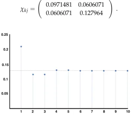
For the example4.4, we obtain the matrixχkjby taking the second derivatives of (15) and evaluate 309
at the parameters found previously, 310
χkj= 0.0971481 0.0606071
0.0606071 0.127964 !
.
Figure 2.Plot of equation (18) for auto-correlation of the observablex02x11with respect to the MEMC consistent with constraintshx1
0x21i=0.1 andhx02x11i=0.3. Here we consider the sum fromr=1 up to
the number in the abscissa. Note the fast convergence towardsχ22.
5.3. Resonances and decay of correlations 311
We turn back to the general setting of an arbitrary ergodic matrixPwith stationary measure
π associated to a Markov chain taking values on a finite state space (not necessarily the space of
spike-patterns). Without loss of generality assume thatPis indexed by the states inE={1, 2, . . . ,M}. It can be proved that in this case there exists(li :i=1, 2, . . . ,M)and(ri:i=1, 2, . . . ,M), sets of left
and right eigenvectors respectively, associated to the eigenvalues(ρi:i=1, . . . ,M). We can assume
that the eigenvectors and left and right eigenvalues have been sorted and normalized in such a way thatρ1=1,l1is the uniqueP–stationary probability vectorπ,r1= (111 . . . 1)T, and
li
rj
whereδi,jis the Kronecker delta, andhu|vi=hu,vicorresponds to the Dirac’s bra-ket,|ui hv|=uvT.
With the same notation, the spectral decomposition ofPis written:
P=
M
∑
i=1
ρi|rii hli| .
Hence:
Pn =
M
∑
i=1
ρni |rii hli| . (20)
Given two functionsf :E7→Randg:E7→Rthe following holds,
Cf,g(n):=Eπ(f(X0)g(Xn))−Eπ(f(X0))Eπ(g(X0)) (21)
=hπ|f ◦Pngi − hπ|fi hπ|gi.
Recall the discussion at previous sections regarding the reverse chain 2.4. Writing E←π for the expectation operator associated to the reverse Markov measure, i.e., to the measureµ=µ(π,←−P), one
can see that
Eπ(f(X0)g(Xn)) =E←π(f(Xn)g(X0)), and hence (21) becomes
D
π
g◦
←−
PnfE− hπ|fi hπ|gi .
From (20)
f ◦Png=
M
∑
i=1
hli|gi |f◦rii
and thus (21) becomes
Cf,g(n) = M
∑
i=1
ρni hli|gi hπ|f◦rii − hπ|fi hπ|gi
=
M
∑
i=2
ρni hli|gi hπ|f◦rii .
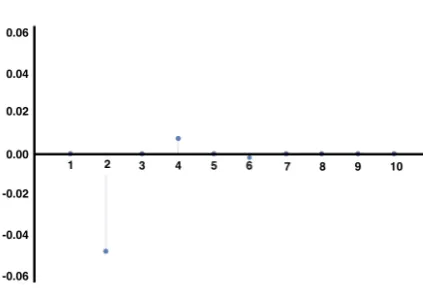
We have found an explicit expression for the decay of correlation for observables from the set of 312
eigenvalues and eigenvectors of the transition matrixP. This is relevant in the context of spike train 313
statistics because as the matrixP characterizing the spike trains is not expected to be symmetric, 314
its eigenvalues are not necessarily real and modulations in the decay of correlations are expected 315
(resonances). When measuring correlations between observables from data, one may observe this 316
Figure 3.Auto-correlations of the observablex02x11for the MEMC with the same parameters as figure 1. We observe modulations in the decay of correlations due to the complex eigenvalues that arise in the non-symmetric transition matrix which is induced by the irreversibility of the MEMC.
5.4. Large deviations for average values of observables in MEMC 318
Obtaining the probability of "rare" average values of firing rates, pairwise correlations, triplets or 319
non-synchronous observables is relevant in spike train statistics as these observables are likely to play 320
an important role in neuronal information processing, and rare values may convey crucial information 321
or be a symptom that the system in not working properly. 322
Here, we build from a previous article [42] where it is shown that the SCGF (7) can be obtained 323
directly from the inferred Markov transition matrixPthrough the Gärtner-Ellis theorem (8). Consider 324
a MEMC with transition matrixP. Let f be an observable of finite range andk∈R. We introduce the 325
tilted transition matrix by f ofP, parametrized bykand denoted byPe(f)(k)[29] as follows: 326
e
Pij(f)(k) =Pijek f(ij) i,j∈S. (22) For MEMCPthe tilted transition matrix can be built directly from the spectral properties of the 327
transfer matrix (12) as follows, 328
e
Pij(f)(k) = e
Hijv j
viρ e k f(ij)
= e
[Hij+k f(ij)]v
j
viρ i,j∈S.
Recall thatvis the right eigenvector associated to its maximum eigenvalueρof the transfer matrixL. 329
Here we also have used the shortcut notationHijto indicate that the energy function is built from the 330
elements of the state spaceiandj. Remarkably, this result is valid not only for the observables in the 331
energy function, i.e., from here the LDP of more general observables can be computed. 332
To obtain an explicit expressions for the SCGFλf(k), is possible to take advantage of the structure 333
of the underlying stochastic process. For instance, for i.i.d. random processXtwhereXi ∼Xfrom the 334
definition7one can obtain that 335
λ(k) = lim t→∞
1 tlnE[e
tkAt(f)]t=ln
E[ek f(X)],
which is the case of range one observables. Using equation (22), we get that the maximum eigenvalue 336
of the tilted matrix, denoted byρ(Pef(k))is, 337
ρ Pef(k)
=
∑
j
SincePef is a positive matrix the Perron-Frobenius theorem ensures the uniqueness ofρ Pef(k)
. 338
For additive observables under the assumption of ergodicity, an straightforward calculation (see for instance [43]) leads us to obtain that
λf(k) =ln ρ Pe(f)
.
It also can be proved thatλf(k), in this case is differentiable [43], setting up the scene to apply the 339
Gärtner-Ellis theorem, which bypasses the direct calculation ofp{AT(f)>s}in (6) throughλf(k)as 340
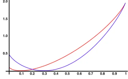
its Legendre transform leads to the rate function of f as shown in figure4. 341
Figure 4.Rate functions of observablesx10x21in red, andx20x11in blue for the MEMC consistent with constraintshx10x12i=0.1 andhx20x11i=0.3. The minimum value of both functions coincide with their expected values with respect to the MEMC. Around the minimum Gaussian fluctuations are expected (9). Far from the expected values are the large deviations.
5.5. Information entropy production 342
Given a Markov chain(Xt:t≥0)on a general finite state spaceEwith transition matrixPstarted
from the distributionν, denoteν(n)the distribution ofXn, namely, fori∈E: ν(n)(i) =Pν(Xn=i).
Obviously,ν(0)=ν, and
ν(jn+1)=
∑
i∈Eνi(n)Pij.
The information-theoretic entropy of the probability distributionνat timenis given by
Sn(ν):=−
∑
i∈Eνi(n)logνi(n),
and thechange of entropyover one time step is defined as ∆Sn :=Sn+1(ν)− Sn(ν).
A bit of algebra yields
∆Sn =−
∑
i,j∈Eν(jn)Pjilog
ν(jn+1)Pji νi(n)Pij
+1
2i,
∑
j∈Eν(jn)Pji−νi(n)Pij
logν
(n)
j Pji νi(n)Pij
The first term on the R.H.S. above is calledinformation entropy flowand the second terminformation 343
entropy production[12]. 344
In the stationary case, i.e., whenPadmits a stationary measureπand the chain is started from
that distribution, one has thatν(n)=πfor everyn≥0; thus, in this case, the change of entropy rate
is zero, i.e., for stationary chains, the information entropy flow equals (minus) information entropy production. This case is the focus on this work. The chain is associated to spike train activity for transitions betweenL–blocks, starting from stationarity we have that the entropy production rate will be explicitly given by
IEP(P,π):= 1
2x,x
∑
0∈SL
π(x0)Px0x−π(x)Pxx0logπ(x
0)P x0x
π(x)Pxx0 ≥0.
The non-negativity implies that information entropy positive as long as the process violate the 345
detailed balance conditions (4). This is analogous to the second law of thermodynamics [44]. From 346
this equation is easy to realize that if the Markov chain satisfies the detailed balance condition the 347
information entropy production is zero. 348
At first glance it may seem contradictory the fact that in stationary state the entropy is constant, 349
but at the same time there is a positive “production” of entropy. In stationary state the information 350
entropy productionalwayscompensate the information entropy flow, thus the information entropy 351
rate remains constant. In this case we refer tonon-equilibrium steady states (NESS). 352
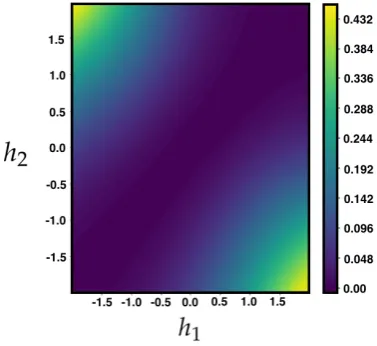
Figure 5.Information entropy production for the MEMC of the example (4.4) for different values of parametersh1,h2. Observe thatIEP(P,π) =0 whenh1=h2and that increases as they become more
different (more asymmetry inP).
5.6. Gallavotti-Cohen fluctuation theorem 353
To characterize the fluctuations of the IEP, consider the MEMC µ(P,π) and the following 354
observable: 355
Wn(x0,n) = 1
nln
µ(x0,n) µ(xn,0)
,
It can be shown that lim1nWn →IEP(π,P). The Gallavotti-Cohen fluctuation theorem is as a 356
statement about properties of the SCGF and rate function of the IEP [14]. 357
This is an universal property of the IEP, i.e., it is independent of the parameters of the MEMC. To 358
computeλW(k)andIW(s), defineA(k)ij=Pij
hπiPij πjPji
ik
. Ifρ(k)is the largest eigenvalue ofA(k), then 359
limn→∞lnE(enλWn) =lnρ(k). 360
This symmetry holds for a general class of stochastic processes including NESS from Markov 361
chains [45]. 362
These properties have an impact on the large deviations of the time-averaged entropy production rate of the sample trajectoryx0,t−1of the Markov chainp(π,P)denoted Wtt. In our framework, the
following relationship always holds,
pnWt t ≈s
o
pnWt t ≈ −s
o e
ts.
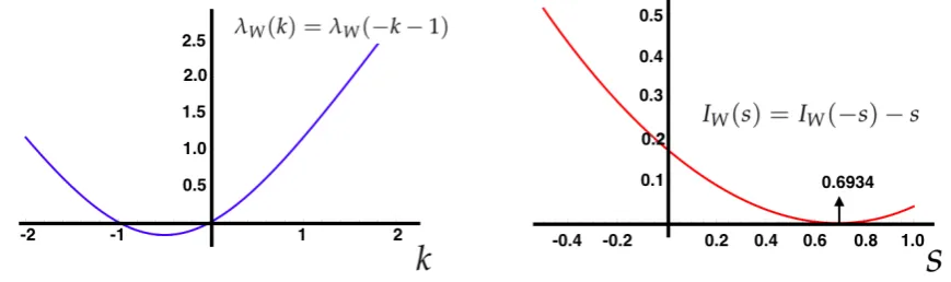
This means that the positive fluctuations of Wt
t are exponentially more probable than negative 363
fluctuations of equal magnitude. 364
Figure 6. Illustration of the Gallavotti-Cohen symmetry property of the large deviation functions associated to the IEP. Left: SCGF of the IEP of the MEMC with the same parameters considered in the previous examples. Right: Rate function of the observableW, the minimum is attained at the expected value of IEP.
5.7. Linear response 365
For a MEMC characterized by µ = (P,π) corresponding to an energy function with fixed 366
parametershdenoted byHh, one can obtain the average value of a given observable fkfrom (16). 367
Now, consider a perturbed energy denoted by ˜H=Hh+δh. Using a Taylor expansion, the average 368
value of an arbitrary observable fkwith respect to the MEMC can be obtained ˜µ= (P˜, ˜π)associated to 369
the perturbed energy 370
The linear response serves to quantify how a small perturbationδh of a set of the maximum 371
entropy parameters affects the average values of observables in terms of the unperturbed measureµ. 372
Considering the Taylor expansion ofF[Hh+δh]aboutHh 373
∂F[Hh+δh]
∂hk
= ∂F[Hh]
hk
+
∑
j
∂2F[Hh] ∂hkhj
δhj+O(δhj)2, (24)
Eµ˜[fk] = Eµ[fk] +
∑
j∂2F[Hh] ∂hkhj
δhj+O(δhj)2, (25)
We use (16) to go from (24) to (25). Observe from (25) that a small perturbation of a parameter 374
hj influences the average value of all other observables in the energy function (as fk is arbitrary). 375
The magnitude of the perturbation is controlled by the second derivatives of the free energy of the 376
unperturbed regimeF[Hh](see figure7). 377
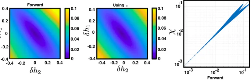
Figure 7.Linear response for the MEMC of the example (4.4) for different values of perturbationsδh1
andδh2. The colors representkEµ˜[fk]−Eµ[fk]kcomputed using two methods. The "forward" method
consist in computingEµ˜[fk]from ˜µandEµ[fk]fromµ. The figure in the middle is obtained computing kEµ˜[fk]−Eµ[fk]kfromχusing equation (26). Right) The difference between both methods illustrated
in a scatter plot in logarithmic scale.
6. Discussion and future work 378
In this work we explore how one can use maximum entropy methods to capture assymetric 379
temporal aspects of biological processes from experimental data. In particular, we showed how 380
spatio-temporal constraints can produce homogeneous irreducible Markov chains whose unique 381
steady state is in general non-equilibrium (NESS) – thus detailed balance condition is not satisfied 382
causing strictly positive entropy production. This fact highlights thatonlynon-synchronous maximum 383
entropy models induce time irreversible processes, which is one of the key hallmark of biological 384
systems. We have presented a survey of diverse techniques from mathematics and statistical mechanics 385
to study these NESS, which correspond to a rich toolkit that can be employed to study unexplored 386
aspects of spike train statistics. Note that although this article is focused on spike train statistics, the 387
discussed tools and methods can be used in other contexts such as ecology, image processing, and 388
economy, among others. 389
Non-equilibrium steady states tools and methods may bring new ideas in the field of 390
computational neuroscience. In particular, possible extensions include measuring the entropy 391
production for different choices of spatio-temporal constraints using the maximum entropy method on 392
biological spike train recordings. A more ambitious extension is to explore the relationship between 393
entropy production of given physiological process and relate them to features such as adaptation or 394
learning. Concerning time-dependent neuronal network models, future studies might lead to a better 395
understanding of the impact of particular synaptic topologies of neuronal network models on the 396
corresponding entropy production, decay of correlations, resonances and other sophisticated statistical 397
properties. 398
Other possible extensions are related to drawbacks of current approaches. This can include 399
limitations of the maximum entropy method related to the requirement of stationarity in the data, which 400
contrast with the fact that information entropy production can still be defined along non-stationary 401
trajectories [14]. Also, another open problem is related to the transfer matrix technique, which currently 402
In summary, we believe that these topics are a fertile ground for multi-disciplinary exploration 404
of teams composed by mathematicians, physicists, and neuroscientists. It is our hope that this work 405
may foster future collaborative research among disciplines, which might bring new breakthroughs to 406
advance our fundamental understanding of how the brain works. 407
Acknowledgments:L.V. is supported by CONICYT-Beca de Doctorado No. 21170406 Convocatoria 2017. F.R.
408
was supported by the Ad Astra Chandaria Foundation. R.C. was supported by CONICYT-PAI Inserción 79160120
409
and Proyecto REDES ETAPA INICIAL, Convocatoria 2017 REDI170457, Fondecyt Proyecto 11181072.
410
Author Contributions: The three authors conceived the main ideas and concepts, wrote and revised the
411
manuscript. All authors have read and approved the final manuscript.
412
Conflicts of Interest:The authors declare no conflict of interest.
413
Abbreviations 414
The following abbreviations are used in this manuscript:
415 416
MEP Maximum entropy principle
MEMC Maximum entropy Markov chain
SCGF Scaled cumulant generating function
CLT Central limit theorem
LLN Law of large numbers
LDP Large deviation principle
IEP Information entropy production
KSE Kolmogorov-Sinai entropy
NESS Non-equilibrium steady states
417
Symbol list 418
S {0, 1}Nthe state space of spike patterns ofNneuron
Ω The set of infinite sequences of spike patterns.
xk
n Spiking state of neuronkat timen.
xn Spike pattern at timen
xt1,t2 Spike block from timet1tot2.
ν(f) Expectation of the observable fw.r.t. the probability measureν.
AT(f) Empirical Average value of the observablefconsideringTspike patterns.
SR Space of spike blocks ofNneurons and lengthR.
S[µ] Entropy of the probability measureµ.
H Energy function.
F[H] Free energy.
419
420
1. Rieke, F.; Warland, D.; de Ruyter van Steveninck, R.; Bialek, W. Spikes, Exploring the Neural Code; M.I.T.
421
Press, 1996.
422
2. Bialek, W.Biophysics: Searching for Principles; Princeton University Press, 2012.
423
3. Schneidman, E.; Berry, M.J.; Segev, R.; Bialek, W. Weak pairwise correlations imply strongly correlated
424
network states in a neural population. Nature2006,440, 1007–12.
425
4. Ganmor, E.; Segev, R.; Schneidman, E. Sparse low-order interaction network underlies a highly correlated
426
and learnable neural population code.Proceedings of the National Academy of Sciences of the United States of
427
America2011,108, 9679–84.
428
5. Tkacik, G.; Marre, O.; Amodei, D.; Schneidman, E.; Bialek, W.; Berry, M.J. Searching for collective behavior
429
in a large network of sensory neurons.PLoS computational biology2014,10, e1003408.
430
6. Palsso, B.Systems Biology: Properties of Reconstructed Networks; Cambridge University Press, 2006.
431
7. Tang, A.; Jackson, D.; Hobbs, J.; Chen, W.; Smith, J.; Patel, H.; Prieto, A.; Petrusca, D.; Grivich, M.; Sher,
432
A.; Hottowy, P.; W.Dabrowski.; Litke, A.; Beggs, J. A Maximum Entropy Model Applied to Spatial and
433
Temporal Correlations from Cortical NetworksIn Vitro. The Journal of Neuroscience2008,28, 505–518.