Scholarship@Western
Scholarship@Western
Electronic Thesis and Dissertation Repository
4-23-2018 10:00 AM
On the Reduction of the Driving Force in Shear-driven Flows
On the Reduction of the Driving Force in Shear-driven Flows
Sakib ShadmanThe University of Western Ontario
Supervisor Floryan, Jerzy M.
The University of Western Ontario
Graduate Program in Mechanical and Materials Engineering
A thesis submitted in partial fulfillment of the requirements for the degree in Master of Engineering Science
© Sakib Shadman 2018
Follow this and additional works at: https://ir.lib.uwo.ca/etd
Part of the Aerodynamics and Fluid Mechanics Commons, Fluid Dynamics Commons, and the Heat Transfer, Combustion Commons
Recommended Citation Recommended Citation
Shadman, Sakib, "On the Reduction of the Driving Force in Shear-driven Flows" (2018). Electronic Thesis and Dissertation Repository. 5289.
https://ir.lib.uwo.ca/etd/5289
This Dissertation/Thesis is brought to you for free and open access by Scholarship@Western. It has been accepted for inclusion in Electronic Thesis and Dissertation Repository by an authorized administrator of
i
In shear-driven flows, an external driving force is needed to maintain the relative movement of horizontal plates. This thesis presents a systematic analysis on using spatially periodic heating and grooved surfaces to control this force. It is found that the use of periodic heating creates a buoyancy-driven effect that always reduces this force. The use of proper heating may even lead to the complete elimination of this force. It is further found that the use of isothermal grooved surfaces always enhances flow resistance, resulting in an increase of this force. When grooves and heating are applied together, their interaction induces a horizontal pressure force that can either increase or decrease the driving force, depending on the relative positions of the groove and heating patterns. Mechanisms leading to such changes of the driving force are discussed.
Keywords
ii
Acknowledgments
Firstly, I would like to thank my supervisor Prof. J. M. Floryan for his precious time and continuous support throughout my Masters. It is difficult to overstate my gratitude to him for his patience, motivation, and enthusiasm. The completion of this work would not have been possible without his immense knowledge, invaluable guidance, incomparable suggestions, and constructive discussions.
I would like to extend my heartiest appreciation to my advisory committee member, Prof. A. G. Straatman for his insightful comments. His curiosities in this project made me think about various aspects and applications of the research outcome.
I am also deeply indebted to Dr. Mohammad Zakir Hossain and Seyed Arman Abtahi. It would have been very difficult for me to finish my Masters without their help. Dr. Hossain has been more than helpful with his precious time for explaining to me the various physical concepts, his suggestions and guidance in writing and his contributions for verifying the results. I would also like to thank Arman for providing the primary framework for the solver and explaining me its potential capacity.
I would also like to thank all my colleagues (past and present), Dr. Hadi Vafadar Moradi, Dr. Alireza Mohammadi, Yanbei Wang for their friendship, cooperation, and helpful attitude.
iii
Table of Contents
Abstract ... i
Acknowledgments ... ii
Table of Contents ... iii
List of Figures ... vi
List of Appendices ... xiv
List of Abbreviations and Nomenclature ... xv
Chapter 1 ... 1
1 Introduction ... 1
1.1 Objective ... 1
1.2 Motivation ... 2
1.3 Related literature survey ... 3
1.3.1 Effects of surface irregularities ... 3
1.3.2 Effects of heating irregularities ... 6
1.4 Outline of the present work ... 9
Chapter 2 ... 10
2 Model Problem ... 10
2.1 Geometry... 10
2.2 Heating pattern ... 11
2.3 Governing equations ... 12
2.4 Boundary conditions ... 13
2.5 Flow constraint... 14
2.6 Reference isothermal case ... 14
2.7 Driving force ... 15
iv
2.9 Heat transfer ... 15
Chapter 3 ... 16
3 Solution procedure ... 16
3.1 Stream function formulation ... 16
3.2 Treatment of the irregular geometry ... 17
3.3 Field equations in the computational plane ... 18
3.4 Discretization of the field equations ... 18
3.5 Discretization of the boundary conditions ... 21
3.6 Discretization of the pressure gradient constraint ... 24
3.7 Numerical solution ... 25
Chapter 4 ... 27
4 Flow between heated smooth parallel plates in relative motion ... 27
4.1 Purely periodic heating at the lower plate... 28
4.2 Plates with unequal mean temperatures ... 39
4.3 Effects of the Prandtl number ... 40
4.4 Heat transfer effects ... 42
4.5 Heating of the upper plate ... 44
4.6 Summary ... 45
Chapter 5 ... 47
5 Flow between grooved isothermal plates in relative motion ... 47
5.1 Flow geometry ... 47
5.2 Driving force applied to the moving plate ... 48
5.3 Sinusoidal grooves ... 49
5.4 Arbitrary grooves ... 52
5.5 Summary ... 56
v
6 Flow between heated grooved plates in relative motion ... 58
6.1 Effects of the phase difference ... 59
6.2 Effects of the wavenumber ... 65
6.3 Effects of the Reynolds number ... 67
6.4 Effects of the groove amplitude ... 69
6.5 Effects of the heating intensity ... 72
6.6 Effects of the plates’ mean temperature... 74
6.7 Effects of the Prandtl number ... 75
6.8 Heat transfer effects ... 77
6.9 Summary ... 80
Chapter 7 ... 81
7 Conclusions and Recommendations ... 81
7.1 Conclusions ... 81
7.2 Future recommendations ... 83
References ... 85
Appendices ... 94
vi
List of Figures
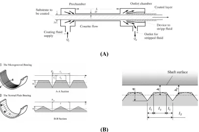
Figure 1-1: Applications of shear-driven flow in (A) coating processes (Figure from (Durst, 2008)), (B) fluid movement in bearings (Figure from (Ashihara & Hashimoto, 2010)). ... 2
Figure 2-1: Schematic diagram of the flow system. ... 11
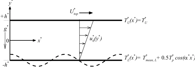
Figure 4-1: Schematic diagram of the flow system ... 27
Figure 4-2: The flow and temperature fields for Rap = 1000, Pr = 0.71, Rauni = 0, α = 2 and
(A) Re = 0, (B) Re = 1, (C) Re = 5, (D) Re = 50. Solid and dashed lines identify streamlines
and isotherms, respectively. Thick streamlines mark borders of bubbles trapping the fluid. Enlargement of the box shown in Figure 4-2B is displayed in Figure 4-3. Flow conditions used in these plots are marked in Figure 4-10 using squares. ... 30
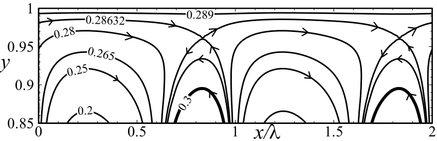
Figure 4-3: Enlargement of the box shown in Figure 4-2B. The streamline emanating from the in-flow stagnation points corresponds to ψ = 0.286322. ... 30
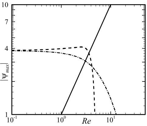
Figure 4-4: Variations of the local |ψmax| associated with the upper plate (solid line), the
clockwise rolls (dashed line), and the counterclockwise rolls (dashed-dotted line) as functions of Re for α = 2, Rap = 1000, Pr = 0.71, Rauni = 0. ... 31
Figure 4-5: Distribution of the shear stress τU acting on the upper plate for α = 2, Rap = 1000,
Pr = 0.71, Rauni = 0 at Re = 1 (solid line) and Re = 10 (dashed line). Enlargement of the box
shown in Figure 4-5A is displayed in Figure 4-5B including shear mean values. ... 32
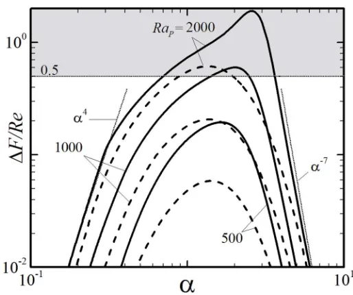
Figure 4-6: Variations of ΔF/Re as a function of α for Pr = 0.71, Rauni = 0, Re = 1 (solid lines)
and Re = 10 (dashed lines). Thin dotted lines identify asymptotes. The shaded area identifies
conditions where the driving force must change direction and becomes a braking force. ... 32
Figure 4-7: The flow and temperature fields for Rap = 1000, Pr = 0.71, Rauni = 0, Re = 1 and α
vii
Figure 4-8: Variations of change of the flow rate driven by movement of the upper plate ΔQ/Re as a function of α for Pr = 0.71, Rauni = 0, Re = 1 (solid lines) and Re = 10 (dashed lines). Thin
dotted lines identify asymptotes. Dashed-dotted line identifies the negative values of ΔQ for
Rap = 2000, Re = 1. ... 34
Figure 4-9: The flow and temperature fields for Rap = 2000, Pr = 0.71, Rauni = 0, Re = 1, α =
0.25. Enlargement of the box in Figure 4-9A is displayed in Figure 4-9B. Thick solid lines identify streamlines, thin solid lines identify negative isotherms while thin dashed lines identify positive isotherms. Thick streamlines mark borders of various bubbles trapping the fluid. .. 35
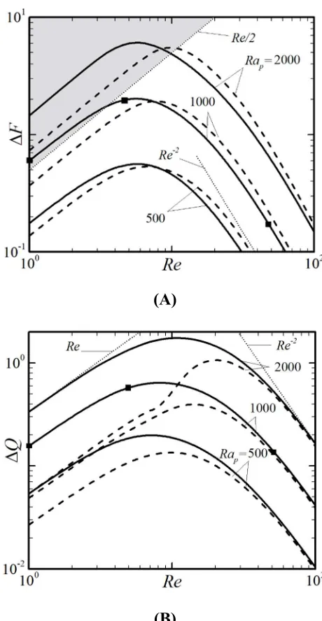
Figure 4-10: Variations of (A) ΔF and (B) ΔQ as functions of Re for Pr = 0.71, Rauni = 0, α
= 2 (solid lines) and α = 1 (dashed lines). Thin dotted lines identify asymptotes. Plots of flow
and temperature field for conditions identified using squares are displayed in Figure 4-2. See text for other details. The shaded area in Figure 4-10A identifies conditions where the driving force must change direction and becomes a braking force. ... 36
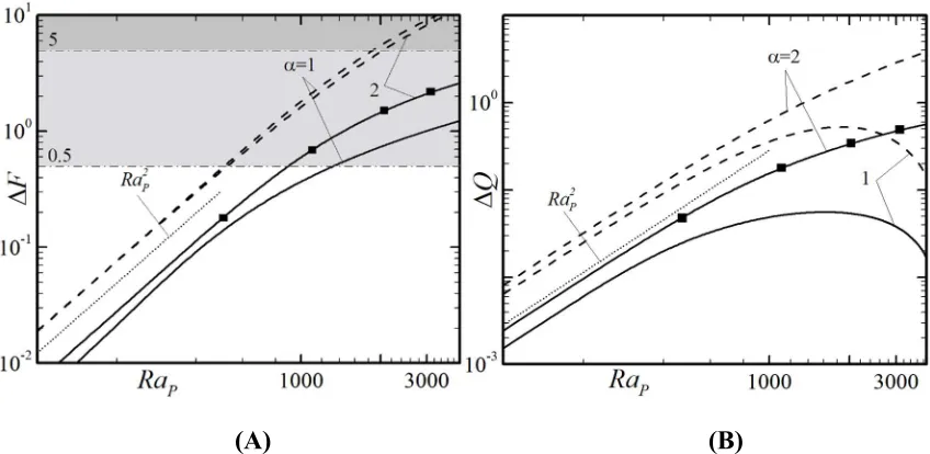
Figure 4-11: Variations of (A) ΔF and (B) ΔQ as functions of Rap for Pr = 0.71, Rauni = 0, Re
= 1 (solid lines) and Re = 10 (dashed lines). Plots of flow and temperature fields for conditions
identified using squares are displayed in Figure 4-12. See text for other details. The shaded area identifies conditions where the driving force must change direction and becomes a braking
force when Re = 1 and the double shaded area identifies such conditions for Re = 10. ... 37
Figure 4-12: The flow and temperature fields for Re = 1, Pr = 0.71, Rauni = 0, α = 2 at (A) Rap
= 500, (B) Rap = 1000, (C) Rap = 2000 and (D) Rap = 3000. Thick solid lines identify
streamlines, thin solid lines identify negative isotherms while thin dashed lines identify positive isotherms. Thick streamlines mark borders of various bubbles trapping the fluid. Flow conditions used in these plots are marked in Figure 4-11 using squares. ... 38
Figure 4-13: Variations of ΔF/Re as a function of (A) α and (B) Rauni for Re = 1 (solid lines)
and Re =10 (dashed lines), and Rap = 1000, Pr = 0.71. The shaded area identifies conditions
where the driving force changes direction and becomes a braking force. ... 40
Figure 4-14: Variations of ΔQ/Re as a function of (A) α and (B) Rauni for Re = 1 (solid lines)
viii
Figure 4-15: Variations of (A) ΔF/Re and (B) ΔQ/Re as functions of Pr at Re = 1 (solid lines) and Re = 10 (dashed lines) for Rap = 1000, Rauni = 0. ... 41
Figure 4-16: Variations of (A) ΔF/Re and (B) ΔQ/Re as functions of α at Re = 1 (solid lines) and Re = 10 (dashed lines) for Rap = 1000, Rauni = 0. ... 41
Figure 4-17: Variations of Nuav in (A) as a function of α for Re = 1 (solid lines) and Re = 10
(dashed lines), in (B) as a function of Re for α = 1 (dashed lines) and α = 2 (solid lines), and in (C) as a function of Rap for Re = 1 (solid lines) and Re = 10 (dashed lines), for Pr = 0.71, Rauni
= 0. Thin dotted lines identify asymptotes. ... 43
Figure 4-18: Variations of Nuav as a function of (A) α and (B) Rauni for Re = 1 (solid lines) and Re = 10 (dashed lines) for Rap= 1000, Pr = 0.71. ... 43
Figure 4-19: Variations of Nuav in (A) as a function of α and in (B) as a function of Pr for Re
= 1 (solid lines) and Re =10 (dashed lines) for Rap = 1000, Rauni = 0. ... 44
Figure 4-20: The flow and temperature fields for the same conditions as in Fig.4-7A but with the upper plate heated and the lower plate moving. Thick solid lines identify streamlines, thin solid lines identify negative isotherms while thin dashed lines identify positive isotherms. Thick streamlines mark borders of bubbles trapping the fluid. ... 45
Figure 5-1: Schematic diagram of the flow system. ... 48
Figure 5-2: Examples of typical flow fields for sinusoidal grooves at the lower plate and smooth upper plate for Re = 100, yb = 0.05. From left to right α = 0.1, 1, 5. ... 49
Figure 5-3:Variations of the difference ΔτU /Re between the shear stresses acting on the upper
smooth plate with the sinusoidal grooves at the lower plate for α = 1, Re = 1 (solid lines) and
Re = 100 (dashed lines). The mean values ΔτU,mean are marked using thin lines. ... 50
Figure 5-4: Variations of (A) ΔF/F0 and (B) ΔQ/Q0 as functions of α for Re = 1 (solid lines)
and 100 (dash-dotted lines). Dotted lines identify asymptotes for α → 0. The upper plate is
ix
Figure 5-5: Variations of (A) ΔF/F0 and (B) ΔQ/Q0 as functions of yb for Re = 1 (solid lines)
and 100 (dash-dotted lines). Thin dotted lines identify asymptotes and the upper bounds. The upper plate is smooth while the lower plate has sinusoidal grooves. ... 52
Figure 5-6: Variations of (A) ΔF and (B) ΔQ as functions of Re for α = 0.1 (dashed lines), α =
1 (solid lines), and α = 5 (dashed-dotted lines).The upper plate is smooth while the lower plate
has sinusoidal grooves. ... 52
Figure 5-7: Geometry of grooves used in the present study. ... 53
Figure 5-8: Variations of ΔF/Re as a function of the number of Fourier modes used for geometry representation for Re = 1, yb = 0.05, α = 1. ... 53
Figure 5-9: Variations of the force increase ΔF for different grooves as functions of (A) yb for Re = 1, α = 1, (B) α for yb = 0.025, Re = 1, (C) Re for yb = 0.025, α = 1. ... 55
Figure 5-10: Variations of the error Er associated with using the first mode of the Fourier expansion representing each groove shape as a function of (A) yb for Re = 1, α = 1, (B) α for yb
= 0.025, Re = 1, and (C) Re for yb = 0.025, α = 1. ... 56
Figure 6-1: Schematic diagram of the flow system. ... 58
Figure 6-2: Evolution of the flow fields as a function of Ω for yb= 0.05, α = 1, Rap = 1000, Re
= 1. Figures (A-H) display results for Ω = 0, π/4, π/2, 3π/4, π, 5π/4, 3π/2, 7π/4, respectively.
Black solid lines identify streamlines associated with the buoyancy-driven rolls while black dashed lines identify streamlines associated with the net flow in the horizontal direction. Grey solid and dashed lines identify the positive and negative isotherms. The lower plate temperature distribution is shown below each figure. Enlargements of boxes marked using dotted lines in Figures (F-H) are shown in Figure 6-3. ... 60
Figure 6-3: Enlargements of the flow fields near the upper plate for (A) Ω = 5π/4, (B) Ω =
3π/2, and (C) Ω = 7π/4. The remaining flow conditions are given in Figure 6-2. ... 61
Figure 6-4: Evolution of the flow field as a function of Ω for yb = 0.05, α = 1, Rap = 1000, Re
x
streamlines, and dashed and dashed-dotted lines identify the positive and negative isobars. Arrows at the lower plate illustrate pressure forces. ... 63
Figure 6-5: Distribution of (A) the x-component σxp,L, and (B) the y-component σyp,L of the
pressure force at the lower plate for yb = 0.05, Re = 1, α = 1, Rap = 1000, and Ω = 0, π/2, 3π/2.
The dashed-dotted line illustrates the no heating conditions. The thick line below each figure
illustrates the groove shape, and dashed and dotted lines illustrate plate temperatures for Ω =
π/2, 3π/2, respectively. ... 63
Figure 6-6: Shear stress distributions at the upper plate (τU) for yb= 0.05, Re = 1, α = 1, Rap=
1000 and Ω = 0, π/2, 3π/2. The thick line below the figure illustrates the shape of the groove,
and dashed and dotted lines illustrate plate temperatures for Ω = π/2, 3π/2, respectively. The
mean values of shear are marked using horizontal lines. ... 64
Figure 6-7: Variations of (A) ΔF/Re and (B) ΔQ/Re as functions of the phase difference Ω for
Rap = 1000, Re = 1, α = 1 and different groove amplitudes. Dashed lines identify results for the
smooth lower plate. The light gray shaded area (zone I) identifies conditions requiring the use of braking force. The white area (zone II) identifies conditions resulting in a reduction of the driving force. The dark gray shaded area (zone III) identifies conditions requiring an increase of the driving force... 65
Figure 6-8: Variations of ΔF/Re as a function of α for yb = 0.01, Rap =1000 and Re = 1, 5 (solid
and dashed lines, respectively). Dotted lines illustrate conditions for the smooth lower plate. The light gray shaded area (zone I) identifies conditions requiring the use of braking force. The white area (zone II) identifies conditions resulting in a reduction of the driving force. The dark gray shaded area (zone III) identifies conditions requiring an increase of the driving force. 66
Figure 6-9: Variations of ΔQ/Re as a function of α for yb = 0.01, Rap =1000 and Re = 1, 5
(solid and dashed lines, respectively). Dotted lines illustrate conditions for the smooth lower plate. ... 66
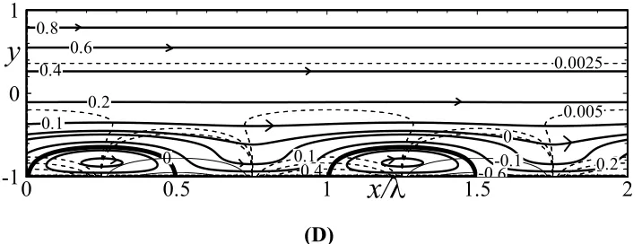
Figure 6-10: Variations of the flow and temperature field for Ω = π/2, Rap = 1000, yb = 1, Re
= 1 for (A) α = 1, (B) α= 2, (C) α= 5, (D) α= 8. Thin dashed and solid lines illustrate the
xi
Figure 6-11: Variations of ΔF as a function of Re for yb = 0.01, Rap = 1000 and α = 2, 3 (solid
and dashed lines, respectively). Dotted lines illustrate results for the smooth lower plate. The light gray shaded area (zone I) identifies conditions requiring the use of braking force. The white area (zone II) identifies conditions resulting in a reduction of the driving force. The dark gray shaded area (zone III) identifies conditions requiring an increase of the driving force. 68
Figure 6-12: Variations of ΔQ as a function of Re for yb = 0.01, Rap = 1000 and α = 2, 3 (solid
and dashed lines, respectively). Dotted lines illustrate results for the smooth lower plate. ... 68
Figure 6-13: Variations of the flow and temperature fields for Ω = π/2, Rap = 1000, yb = 1, α
= 2 for (A) Re = 1, (B) Re = 5, (C) Re = 10, (D) Re = 50. Thin dashed and solid lines illustrate
the positive and negative isotherms. ... 69
Figure 6-14: Variations of ΔF/Re as a function of yb for Rap = 1000, α = 2, Re = 1, 5 (solid and
dashed lines, respectively). Dotted lines illustrate the solution for the smooth plate. The light gray shaded area (zone I) identifies conditions requiring the use of braking force. The white area (zone II) identifies conditions resulting in a reduction of the driving force. The dark gray shaded area (zone III) identifies conditions requiring an increase of the driving force. ... 70
Figure 6-15: Variations of ΔQ/Re as a function of yb for Rap = 1000, α = 2 and Re = 1, 5 (solid
and dashed lines, respectively). Dotted lines illustrate solutions for the smooth lower plate. 70
Figure 6-16: Variations of the flow and pressure fields for Ω = π/2, Rap = 1000, α = 1, Re = 1
for (A) yb = 0.001, (B) yb= 0.025, and (C) yb = 0.05. Thin dashed and solid lines illustrate the
positive and negative isobars. ... 71
Figure 6-17: Variations of the x-component of the induced pressure force for the flow fields shown in Figure 6-16(A-C). ... 71
Figure 6-18: Variations of ΔF/Re as a function of Rap for yb = 0.01, α = 2 and Re = 1, 5 (solid
xii
Figure 6-19: Variations of ΔQ/Re as a function of Rapfor yb = 0.01, α = 1 and Re = 1, 5 (solid
and dashed lines, respectively). Dotted lines identify results for the smooth lower plate. Grey lines identify negative values. Figure (A) displays results in the log-log scale while Fig. (B) uses the semi-log scale. ... 73
Figure 6-20: Variations of the flow and temperature fields for Ω = π/2, yb = 1000, α = 1, Re =
1 for (A) Rap= 100, (B) Rap = 500, (C) Rap = 1000, (D) Rap = 2000. Thin dashed and solid
lines identify the positive and negative isotherms. ... 73
Figure 6-21: Variations of ΔF/Re for Rap= 1000, yb = 0.01 as a function of (A) Rauni for α = 1
and (B) α for Re = 1. In (A), solid and dashed lines correspond to Re = 1, 5, respectively. In
(B), dashed, solid and dashed-dotted lines correspond to Rauni = -150, 0, 150, respectively.
Dotted lines identify results for the smooth lower plate. The light gray shaded area (zone I) identifies conditions requiring the use of braking force. The white area (zone II) identifies conditions resulting in a reduction of the driving force. The dark gray shaded area (zone III) identifies conditions requiring an increase of the driving force. ... 74
Figure 6-22: Variations of ΔQ/Re for Rap = 1000, yb = 0.01 as a function of (A) Rauni for α = 1
and (B) α for Re = 1. In (A), solid and dashed lines correspond to Re = 1, 5, respectively. In
(B), dashed, solid and dashed-dotted lines correspond to Rauni = -150, 0, 150, respectively.
Dotted lines identify results for the smooth lower plate. ... 75
Figure 6-23: Variations of ΔF/Re as a function of Pr for yb= 0.01, Rap= 1000, α = 2 at Re =
1, 5 (solid and dashed lines, respectively). Figure (A) displays results in the log-log scale while Fig. (B) uses the semi-log scale. In (A), dashed-dotted lines identify negative values. Dotted
lines are used to identify results for the smooth lower plate at Re = 1. The light gray shaded
area (zone I) identifies conditions requiring the use of braking force. The white area (zone II) identifies conditions resulting in a reduction of the driving force. The dark gray shaded area (zone III) identifies conditions requiring an increase of the driving force. ... 76
Figure 6-24: Variations of ΔQ/Re as a function of Pr for yb= 0.01, Rap= 1000, α = 2 at Re =
xiii
Figure 6-25: Variations of (A) ΔF/Re, and (B) ΔQ/Re as function of α for yb= 0.01, Rap =
1000, Re = 1 and Pr = 0.71, 1, 5 (solid, dashed-dotted and dashed lines, respectively). Dotted
lines identify conditions for the smooth lower plate. The light gray shaded area (zone I) identifies conditions requiring use of braking force. The white area (zone II) identifies conditions resulting in a reduction of the driving force. The dark gray shaded area (zone III) identifies conditions requiring an increase of the driving force. ... 77
Figure 6-26: Variations of Nuavas a function of (A) Ω and (B) α. In (A), Rap= 1000, α = 1, Re
= 1. In (B), Rap= 1000, yb= 0.01, Re = 1, 5 (solid and dashed lines, respectively). Dotted lines
illustrate conditions for the smooth lower plate. ... 78
Figure 6-27: Variations of Nuavas a function of (A) Re, (B) Rap, (C) yb. In (A), Rap= 1000, α
= 2 (solid lines) and α = 3 (dashed lines), yb = 0.01. In (B), yb = 0.01, α = 2, Re = 1 (solid lines)
and Re = 5 (dashed lines). In (C), Rap= 1000, α = 2, Re = 1 (solid lines) and Re = 5 (dashed
lines). Thin dotted lines identify asymptotes. ... 78
Figure 6-28: Variations of Nuav as a function of (A) Rauni, and (B) α. In (A), yb= 0.01, Rap=
1000, α = 2, Re = 1 (solid lines) and Re = 5 (dashed lines). In (B), yb = 0.01, Rap= 1000, Re =
1, Rauni = -150 (dashed lines), Rauni= 0 (solid lines), and Rauni = 150 (dashed-dotted lines).
Dotted lines illustrate results for the smooth lower plate. ... 79
Figure 6-29: Variations of Nuav as a function of (A) Pr, and (B) α. In (A), yb = 0.01, Rap =
1000, α = 2, Re = 1 (solid lines) and Re = 5 (dashed lines). In (B), yb= 0.01, Rap = 1000, Re =
1, Pr = 0.71 (solid lines), Pr = 1 (dashed-dotted lines), and Pr = 5 (dashed lines). Dotted lines
xiv
List of Appendices
Appendix A: Recurrence formulae and Chebyshev inner products... 94
xv
List of Abbreviations and Nomenclature
Abbreviations
RB Rayleigh – Bénard
IBC Immersed Boundary Conditions
RF Relaxation Factor
Nomenclature
Chapter 1
Ra Rayleigh number = ∆
Racr Critical Rayleigh number for the onset of the
Rayleigh – Bénard instability
Re Reynolds number =
Chapter 2
* Superscript denoting dimensional quantities
0 Subscript denoting reference case
c Specific heat
F Driving force
g Gravitational acceleration
xvi
k Thermal conductivity
L Subscript denoting lower plate
mean Subscript denoting mean value
Nu Nusselt number =
p Subscript denoting periodic value
p Pressure
Pr Prandtl number =
Q Flow rate
T Temperature
U Subscript denoting upper plate
(u, v) Velocity component in the (x, y) direction
uni Subscript denoting uniform value
(x, y) Physical coordinate system
yb Amplitude of the groove at the lower plate
yU, yL Shapes of the upper and lower plates in the
physical coordinate system
α Wavenumber
Г Thermal expansion coefficient
θ Relative temperature
xvii
λ Wavelength
μ Dynamic viscosity
ν Kinematic viscosity
ρ Density
τ Shear stress
Ω Phase difference
Chapter 3
* Superscript denoting complex conjugates
〈𝑛〉 Superscript denoting Fourier mode
A Mean pressure gradient
𝐴( ) Coefficients of Fourier expansions describing
the geometry
D Derivation with respect to transverse direction
𝐷𝐿( ) Coefficients of the Fourier expansions for the
first derivative of the Chebyshev polynomials evaluated at the lower plate
𝐺𝜑 Chebyshev coefficients in the expansion
representing 𝜑( )
xviii
representing velocity and temperature products
𝐺∅ Chebyshev coefficients in the expansion
representing ∅( )
i Imaginary part
l Iteration number
NM Number of Fourier modes used for
discretization in the x – direction
NS Number of Fourier modes used to describe the
Chebyshev polynomials and their derivatives evaluated at the upper and lower plates
NT Number of Chebyshev polynomials used for
discretization of the modal function in the 𝑦-
direction
NVV, NVθ Nonlinear terms
Nx Number of grid points along the x- direction
in (x,𝑦) plane
Tk k-th Chebyshev polynomial of the first kind
𝑢𝑢, 𝑢𝑣, 𝑣𝑣, 𝑢𝜃, 𝑣𝜃 Velocity and temperature products in the physical space
𝑢𝑢( ), 𝑢𝑣( ), 𝑣𝑣( ), 𝑢𝜃( ), 𝑣𝜃( ) Modal functions of the velocity and
temperature products 𝑢𝑢, 𝑢𝑣, 𝑣𝑣, 𝑢𝜃, 𝑣𝜃
𝑊𝐿( ) Coefficient of Fourier expansion for the
xix
(x,𝑦) Coordinate system in the computational
domain
𝛤 Constant associated with the transformation
for the IBC method
∅( ) Modal functions in the Fourier expansion
representing the temperature
𝜑( ) Modal functions in the Fourier expansion
representing the stream function
ψ Stream function
Chapter 1
1
Introduction
In simple shear-driven flows, the relative movement between two parallel plates drives the fluid flow. These flows are characterized by the absence of a streamwise pressure gradient. An external force is required to maintain the relative plate movement. There is an interest in the reduction of this external force as this would lead to the reduction of the energy expenditure associated with operations of such systems. This reduction of the driving force is analogous to the drag reduction in other systems. Common techniques of drag reduction
include injection of dilute polymers (Bonn, et al., 2005), introduction of plate oscillations
(Hurst, et al., 2014), use of suction/blowing (Segawa, et al., 2007; Virk, 1975), use of various actuators (Mahfoze & Laizet, 2017), use of heating patterns (Hossain & Floryan, 2016), and changing the plate topography (Mohammadi & Floryan, 2013b), to name a few. Some of these approaches can be characterized as focused on the laminar flow control so that transitions to secondary states are avoided. Others, like the one which is followed in this thesis, are focused on the creation of spatial flow modulations which would lead to the reduction of shear and, thus, reduction of the frictional resistance.
1.1
Objective
1.2
Motivation
Shear-driven flows have been of interest since the works of Couette in the early nineteenth century. Since then, this class of flows has been widely used in industry. Applications include processes like coating (Weinstein & Ruschak, 2004) (see Figure 1-1A), fluid movement in bearings and between shafts (see Figure 1-1B), fluid sealing systems, lubrication problems, towing of free-floating bodies in shallow basins, etc. Further applications can be identified in Micro-Electro-Mechanical-Systems (Ho & Tai, 1998) and in chemical processes (Desmet & Baron, 2000).
The boundary and temperature irregularities frequently occur in nature, e.g. air circulation in the atmospheric boundary layer and heat island effect, mixing in oceans, shark skins which allow them to move with a particular ease, compact heat exchangers, microfluidic and nanofluidic devices, cell analyzers, and many others.
(A)
(B)
Most of the existing studies dealing with surface and temperature irregularities are focused on the pressure-driven flows. Therefore, there exists a void in knowledge regarding flow responses due to surface irregularities and heating patterns in shear-driven flows. Given their frequent use in industries, the development of techniques to control the costs required to maintain such flows provides the main motivation for this study.
1.3
Related literature survey
There exists a considerable number of analyses dealing with the effects of surface irregularities, but they are mostly focused on the pressure-driven flows. Likewise, the existing literature dealing with the effects of heating is mostly focused on the convective heat transfer. Therefore, the discussion of the literature is divided into several categories, with each of them focused on a specific issue of interest in this analysis.
1.3.1
Effects of surface irregularities
1.3.1.1
Pressure-driven flows
The effect of geometric irregularity (surface roughness) in pressure-driven flows is a classical yet not fully understood concept in fluid mechanics. The history of studying the effects of surface roughness dates back to the works of Darcy (1857) and Hagen (1854), who concluded that roughness always increases the overall flow resistance. Moody (1944) and Nikuradse (1933), with the limited instrumentation available at that time, carried out extensive experiments and proposed the concept of friction factor for drag quantification. They also concluded that the drag in laminar flow is independent of surface roughness or, at least, roughness effects were too small to be determined using the existing measuring techniques. These correlations suggest that surface roughness has a significant effect on the turbulent flow and always increases the turbulent drag.
reduce the drag below what is found for smooth plates. These special surface shapes were referred to as riblets, i.e. short wavelength streamwise grooves. Effects of riblets on drag
reduction were further studied experimentally by Walsh & Lindemann (1984), Bruse, et
al. (1993), Bechert, et al. (1997), and numerically by Choi, et al. (1991), Chu & Karniadakis (1993), Chu, et al. (1992), Goldstein & Tuan (1998), Goldstein, et al. (1995), and in all of these cases it was concluded that riblets were capable of reducing turbulent drag but no clear conclusion was reached about the laminar drag.
Pressure losses for laminar flows over geometric irregularities gained interest due to the occurrence of such flows in micro and nano-channels, and due to deviation from the
classical theories based on the works of Gamrat et al. (2008), Papautsky et al. (1999), Sharp
& Adrian (2004), and Sobhan & Garimella (2001). Mohammadi & Floryan (2013b) investigated pressure loss in grooved channels for laminar flows and found potential to obtain drag reduction by the proper shaping of grooves. Mohammadi (2013), Mohammadi & Floryan (2013a), Moradi (2014), and Moradi & Floryan (2013) investigated longitudinal grooves and quantified their drag reducing abilities.
Mohammadi & Floryan (2012) categorized the mechanisms responsible for the generation of drag into three types, namely associated with the pressure form drag, the pressure interaction drag, and the shear drag. The shear drag is associated with surface-groove-induced changes in the wall shear, as well as with an increase of the wetted area. The pressure form drag is associated with the mean pressure gradient driving the flow and the pressure interaction drag is generated through an interaction between the groove-modulated part of the pressure field and the surface geometry. The importance of pressure effects increases rapidly with the groove amplitude. Information about the types of drag and their dependence on the groove shape offers potential for identification of surface topographies that may result in a lower drag.
Use of the superhydrophobic effect is also useful in reducing drag. In this case, the surface topography traps gas bubbles in micro-pores, replacing the shear stress between liquid and solid with a shear stress between liquid and gas (Rothstein, 2010). Existence of the laminar
(2004), Ou & Rothstein (2005) and Truesdell, et al. (2006). The effectiveness of this
method was optimized by correctly shaping the surface pores (Samaha, et al., 2011) and
by changing the hydrophobicity using changes in the surface chemistry (Quere, 2008;
Reyssat, et al., 2008; Zhou, et al., 2011). The stability characteristics in such flows are not
yet fully understood.
1.3.1.2
Shear-driven flows
The plane-Couette flow represents the simplest shear-driven flow. It occurs between two parallel plates in relative motion. It is characterized by the lack of a streamwise pressure gradient as the flow is driven by plate movement only. The flow has linear velocity distribution and constant shear throughout the flow field. It is also linearly stable (Romanov, 1972). The transition to secondary states has been studied in detail by Deguchi & Nagata (2011) who identified various routes to secondary finite-amplitude states as well as to turbulence.
The experiments on transition between the laminar and turbulent states and the role of roughness in Couette flow are described in Aydin & Leutheusser (1991). The form of the
flow is predicted analytically for long wavelength grooves in Malevich, et al. (2008). The
potential slip at the rough surface is discussed in Niavrani & Priezjev (2009), and Priezjev & Troian (2006). While it is known that Couette flow is linearly stable (Romanov, 1972), it becomes unstable in the presence of grooves resulting in the formation of streamwise vortices (Floryan, 2002). Similar secondary flows may appear due to the introduction of wall transpiration (Floryan, 2003). Shear instability modes are generated in the annular Couette flow (Moradi & Floryan, 2013). Various simplified models have been used to
study effects of varying groove geometry (Sahlin, et al., 2005; Valdés, et al., 2012; Wang,
1.3.2
Effects of heating irregularities
A recently introduced technique for drag reduction uses spatial heating patterns (Hossain
& Floryan, 2016)that create a buoyancy field which leads to the formation of a system of
separation bubbles. Fluid trapped inside these bubbles rotates due to the action of horizontal density gradients and as a result, a propulsive force is created which contributes to fluid pumping. In addition, these bubbles isolate the stream from direct contact with the plate and thus reduce the frictional drag. This phenomenon is referred to as the super-thermo-hydrophobic effect (Floryan, 2012). This effect is enhanced by combining distributed and uniform heating of the lower plate (Floryan & Floryan, 2015). Similar results can also be achieved by heating the upper plate (Hossain & Floryan, 2014). One drawback of this technique lies in the fact that the flow has to be fairly slow as stronger
flows wash away separation bubbles (Hossain, 2011; Hossain, et al., 2012; Hossain &
Floryan, 2015). This limitation leads to the search for ways of enhancing this effect so that
it can be applied at higher Reynolds numbers. Yamamoto, et al. (2013) demonstrated
simultaneous drag reduction and heat transfer enhancement using suction/blowing waves travelling in the downstream direction. Their results provide motivation for exploring these methods in conjunction with the heating non-uniformities. However, when both plates were heated, drag reduction strongly depended on the phase difference between the lower and upper heating. The drag reduction could increase by up to three times over that found in the case of one plate heating if the proper phase difference was used. The range of Reynolds numbers with effective drag reduction was doubled at the same time (Hossain & Floryan, 2016).
Heating non-uniformities represent a wider class of problems which have been studied on a case by case basis and not necessarily in the context of drag reduction. The non-uniformities create horizontal and vertical temperature gradients which result in the horizontal density variations that create motions referred to as horizontal convection. Maxworthy (1997) reviewed the numerical and experimental analyses focused on
convection in regions with either open or partially-open lateral boundaries. Siggers, et al.
differentially at its surface with a general temperature distribution imposed at the top of the layer and a variety of thermal boundary conditions at the base of the layer. Hughes & Griffiths (2008) used horizontal convection as an idealized model of the ocean overturning circulation with the non-uniform heating profiles imposed at a horizontal boundary and demonstrated that convection depends on the geometry of the flow system and on the externally imposed thermal conditions.
The analyses of fundamental aspects of convection have been focused on simple reference cases as many variables affect the system response. Consider the simplest case of a horizontal slot subject to a spatially homogeneous heating applied at the lower plate, also known as the Rayleigh-Bénard (RB) convection (Bénard, 1900; Rayleigh, 1916). This convection results from the transition from a conductive state when the critical conditions
are exceeded and it changes the character of the heat flow in qualitative terms (Ahlers, et
al., 2009; Bodenschatz, et al., 2000; Chilla & Schumacher, 2012; Lohse & Xia, 2010).
These critical conditions are expressed in terms of the critical Rayleigh number Racr with
secondary flow occurring for Ra > Racr. A large enough heating intensity leads to turbulent
RB convection (Ahlers et al., 2009; Lohse & Xia, 2010). Convection onset conditions are
affected by the heating non-uniformities (Freund, et al., 2011) as well as geometric
non-uniformities (McCoy, et al., 2008; Seiden, et al., 2008; Weiss, et al., 2012). Results dealing
with the effects of geometry modulation on the RB convection are very limited but demonstrate that the non-uniformities do play a role. Two-dimensional convection rolls
have been observed for subcritical conditions (Ra << Racr) in the case of the lower plate
being augmented with thin stripes. The amplitude of these rolls grew with Ra until they
were destabilized with mechanisms which depended on the ratio of the wavenumber of the imposed modulation and the critical wavenumber of the RB convection producing a variety of three-dimensional patterns.
There exist several studies focused on the applied aspects of convection and involving specialized geometries. Bergeles (2001) showed that for single phase flows in tubes, up to a 400% increase in the nominal heat transfer coefficient can be achieved by adjusting
surface topography. Siddique, et al. (2011) reviewed different heat transfer enhancing
porous media, suspensions of large particles, suspensions of small particle (nanofluids), phase-change devices, flexible seals, vortex generators, protrusions, composite materials with ultra-high thermal conductivity, etc. Ligrani, et al. (2003) suggested that all these techniques can either create secondary flows and/or can increase the turbulence level
resulting in an increase of fluid mixing. Dewan, et al. (2004) reviewed the passive heat
transfer augmentation techniques based on the use of twisted tapes and wire coils. There exists a lack of fundamental and systematic research on the effects of surface roughness/grooves on natural and mixed convection, and on the onset of secondary states in buoyancy-driven motions. This becomes more eminent in micro-channels where the roughness size cannot be reduced to a negligible level using the currently available manufacturing techniques. Sobhan & Garimella (2001) reviewed different studies on the flow and heat transfer in micro-channels with surface roughness and concluded that there is a need for additional systematic studies to examine the effects of each of the concerned
parameters separately. Xia et al. (2011) studied the fluid flow and heat transfer mechanisms
in micro-channels and concluded that change in surface area and complexities in the boundary layer were primarily responsible for change in heat transfer characteristics with a change in the pressure drop.
Recently, Toppaladoddi et al. (2015) studied geometric optimization for heat
pressure forces depended on the groove geometry, location and the heating conditions. The changes in the heat flow were quite complex as they resulted from a combination of conductive changes associated with grooves and convective changes associated with the heating and geometric irregularities.
Abtahi & Floryan (2017a, b) analyzed natural convection in a horizontal fluid layer exposed to heating and geometric irregularities. They considered periodic distribution for both heating and geometric irregularities and quantified their relative position using phase difference. They concluded that the interaction of the heating and groove patterns was able to create a net horizontal flow in the absence of any mean pressure gradient. This flow could be directed in any direction depending on the phase difference between the heating and groove patterns.
1.4
Outline of the present work
Chapter 2
2
Model Problem
This chapter describes the model problem which captures the physical phenomenon of interest in the analysis, i.e. reduction of forces required to support the relative movement of parallel plates. Spatially distributed heating is the method of choice for force reduction. This heating is applied to the stationary plate, which can be grooved, while the moving plate is kept isothermal and smooth. The model problem is two-dimensional as the force reducing method is two-dimensional. It is assumed that the working fluid is Newtonian, and its properties are well described using Boussinesq approximation. Section 2.1 depicts the general geometry to be considered, Section 2.2 describes the external heating pattern to be applied, Section 2.3 provides a concise summary of the governing equations to be used, Sections 2.4 and 2.5 discuss the relevant boundary conditions and the flow constraint. A reference isothermal case is explained in Section 2.6. Evaluation of forces, flow rate and induced heat transfer are discussed in Sections 2.7-2.9.
2.1
Geometry
Consider two horizontal plates moving relative to each other with the gap between them filled with a fluid. The upper plate is smooth while the lower one is assumed to be sinusoidally grooved resulting in the gap geometry of form –
𝑦∗(𝑥∗) = −ℎ∗+ 𝑦∗ 𝑐𝑜𝑠(𝛼∗𝑥∗), (2.1a)
𝑦∗(𝑥∗) = ℎ∗. (2.1b)
where the subscripts L and U refer to the lower and upper plates respectively, 𝑦∗ is the
amplitude of the groove, 𝛼∗ is its wavenumber and stars identify dimensional quantities.
The gap extends to ±∞ in the x*-direction, its mean opening is 2ℎ∗, and its periodicity is
Considering the half of the mean gap height ℎ∗ as the length scale, the dimensionless form
of the gap geometry becomes
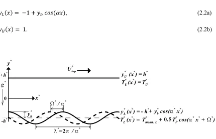
𝑦 (𝑥) = −1 + 𝑦 𝑐𝑜𝑠(𝑥), (2.2a)
𝑦 (𝑥) = 1. (2.2b)
Figure 2-1: Schematic diagram of the flow system.
2.2
Heating pattern
Introduce an external heating resulting in sinusoidal temperature variations along the lower plate and a constant temperature of the upper plate, i.e.
𝑇∗(𝑥∗) = 𝑇 ,
∗ + 0.5 𝑇∗ 𝑐𝑜𝑠(𝛼∗𝑥∗+ Ω∗), (2.3a)
𝑇∗(𝑥∗) = 𝑇∗, (2.3b)
where the subscripts “mean” and “p” refer to the mean and periodic parts, respectively,
𝑇∗ is the peak-to-peak amplitude of the periodic component, and 𝛺∗is the phase shifts
between the heating and groove patterns. Use of the upper plate temperature for reference (all material properties are to be evaluated at this temperature) and introduction of the
relative temperature ∗ = 𝑇∗ – 𝑇∗ lead to plates’ temperatures of the form
0
-h*
+ h* y
U
* (x*) =
TU*(x*) =
yL*(x*) = TL*(x*) = T*
mean, L+
U* top
g*
x*
y*
h* TU*
0.5
+ yb*cos(*
x*) - h*
yb*
*/*
*
= /*
2
T*
Pcos(
𝜃∗(𝑥) = 𝜃∗ + 0.5 𝜃∗ 𝑐𝑜𝑠(𝛼∗𝑥∗+ Ω∗), (2.4a)
𝜃∗(𝑥) = 0. (2.4b)
where 𝜃∗ = 𝑇∗ , − 𝑇∗, and 𝜃∗ = 𝑇∗.
Considering 𝜅∗𝜈∗⁄(𝑔∗𝛤∗ℎ∗ ) as the temperature scale results in the following
dimensionless expression for the temperatures of the plates
𝜃 (𝑥) = 𝑅𝑎 + 0.5 𝑅𝑎 𝑐𝑜𝑠(𝛼𝑥 + Ω), (2.5a)
𝜃 (𝑥) = 0 (2.5b)
where 𝑅𝑎 = 𝑔∗𝛤∗ℎ∗ 𝑇∗ ⁄(𝜅∗𝜈∗) is the uniform Rayleigh number measuring the
intensity of the uniform (mean) part of the applied heating and 𝑅𝑎 = 𝑔∗𝛤∗ℎ∗ 𝑇∗⁄(𝜅∗𝜈∗)
is the periodic Rayleigh number measuring the intensity of the periodic part of the applied heating.
2.3
Governing equations
Assume that the upper plate is pulled in the positive x*-direction with a constant velocity
𝑈∗ while the lower plate is stationary. The fluid is assumed to have thermal conductivity
𝑘∗, specific heat 𝑐∗, thermal diffusivity 𝜅∗ = 𝑘∗⁄𝜌∗𝑐∗, kinematic viscosity 𝜈∗, dynamic
viscosity μ∗, thermal expansion coefficient 𝛤∗ and variations of its density 𝜌∗ follow the
Boussinesq approximation. The gravitational acceleration 𝑔∗ is acting in the negative y*
-direction.
Considering the velocity scale to be 𝑈 ∗ = 𝜈∗⁄ℎ∗ and the pressure scale to be 𝜌∗𝑈∗ , the
dimensionless field equations take the following form:
+ = 0, (2.6a)
𝑢 + 𝑣 = − + ∇ 𝑣 + 𝑃𝑟 𝜃, (2.6c)
𝑢 + 𝑣 = 𝑃𝑟 ∇ 𝜃 (2.6d)
where (𝑢, 𝑣) are the velocity components in the (x, y) directions, respectively, 𝑝 stands for
the pressure, denotes the temperature and Pr = 𝜈∗/𝜅∗ is the Prandtl number.
2.4
Boundary conditions
The system (2.6) is subject to the following boundary conditions
(i) The no-slip conditions:
𝑢(𝑦 (𝑥)) = 0, (2.7a)
𝑢(1) = 𝑅𝑒 (2.7b)
where Re is the Reynolds number defined as 𝑅𝑒 = 𝑈∗ /𝑈 ∗ = 𝑈∗ ℎ∗/𝜈∗.
(ii) The no-penetration conditions:
𝑣(𝑦 (𝑥)) = 0, (2.7c)
𝑣(1) = 0. (2.7d)
(iii) The thermal conditions:
𝜃(𝑦 (𝑥)) = (𝑥), (2.7e)
2.5
Flow constraint
No mean horizontal pressure gradient is permitted in the flow system, hence one must impose constraint of the form
= 0. (2.8)
2.6
Reference isothermal case
When the above system is isothermal, and both plate surfaces are smooth, the fluid movement in the gap is solely caused by the motion of the upper plate, and is given as
𝒗 (𝑥, 𝑦) = [𝑢 (𝑦), 0] = (1 + 𝑦), 0 , (2.9a)
𝑝 (𝑥, 𝑦) = 𝐶. (2.9b)
The fluid flow rate in the gap is
𝑄 = 1, (2.9c)
the shear stress acting on the upper plate is
𝜏 = −0.5. (2.9d)
and the force (per unit length and unit width) required to pull the upper plate is given as
𝐹 = 0.5. (2.9e)
In the above, the velocity vector 𝒗𝟎 has been scaled with 𝑈∗ as the velocity scale, Q0
stands for the flow rate scaled with the same velocity scale, 𝜏 stands for the shear acting
on the upper plate scaled with 𝑈∗ 𝜇∗/ℎ∗, 𝐹 denotes the force per unit length and width
2.7
Driving force
Certain force must be applied to the upper plate to maintain its movement, and the magnitude of this force is determined by shear forces acting on its surface.
The presence of the grooves and the heating results in changes in the shear stress acting on
the upper plate, ∆𝜏∗ = 𝜏∗− 𝜏∗, which, when scaled with 𝑈∗𝜇∗/ℎ∗, has the form
∆𝜏 = − + 𝑅𝑒. (2.10)
The change in the driving force, ∆𝐹∗ = 𝐹∗− 𝐹∗, scaled with 𝜌∗𝑈∗ , can be expressed as
∆𝐹 = 𝐹 − 𝐹 = 𝑅𝑒 − 𝑅𝑒 𝜆 ∫ 𝑑𝑥 . (2.11)
2.8
Flow rate
The change in the amount of fluid pulled by the plate, ∆𝑄∗ = 𝑄∗− 𝑄∗, scaled with 𝑈 ∗,
can be expressed as
∆𝑄 = 𝑅𝑒 𝑅𝑒 ∫ 𝑢(𝑥, 𝑦) 𝑑𝑦 − 1 . (2.12)
2.9
Heat transfer
The external heating required to produce the desired temperature along the lower plate leads to a heat flow between the plates which can be viewed as an energy cost associated with the use of the heating for altering the driving force. This heat flow is expressed in terms on the mean Nusselt number defined as
Chapter 3
3
Solution procedure
This chapter focuses on describing the procedure used for the determination of a solution for the problem presented in Chapter 2. It describes the discretization procedure for the field equations and boundary conditions, and the efficient solution process for solving these equations. The solution method presented in this chapter is based on the method described
by Abtahi, et al. (2016) and Husain & Floryan (2013).
3.1
Stream function formulation
The field equations presented in Section 2.3 are to be expressed in terms of the stream
function ψ defined as
𝑢 = , 𝑣 = − . (3.1)
The above definition of stream function automatically satisfies the continuity equation (2.6a) and facilitates elimination of the pressure terms from the momentum equations (2.6b-c). The field equations take the following final form
∇ 𝜓 − 𝑃𝑟 = 𝑁 , (3.2a)
∇ 𝜃 = 𝑃𝑟𝑁 (3.2b)
where the nonlinear terms NVV and NVθ are defined as
𝑁 = 𝑢𝑢 + 𝑢𝑣 − 𝑢𝑣 + 𝑣𝑣 , (3.3a)
𝑁 = 𝑢𝜃 + 𝑣𝜃. (3.3b)
The boundary conditions (2.7a-f) expressed in terms of the stream function assume the following forms
𝑦 (𝑥) = 0, (3.4a)
𝑦 (𝑥) = 𝑅𝑒, (3.4b)
𝑦 (𝑥) = 0, (3.4c)
𝑦 (𝑥) = 0, (3.4d)
𝜃 𝑦 (𝑥) = 𝜃 (𝑥), (3.4e)
𝜃 𝑦 (𝑥) = 𝜃 (𝑥). (3.4f)
3.2
Treatment of the irregular geometry
The geometric irregularity of the flow domain is taken care of by using the Immersed Boundary Conditions (IBC) (Mittal & Iaccarino, 2005; Peskin, 2002; Szumbarski & Floryan, 1999) concept where a fixed rectangular computational domain is used that is sufficiently large to contain the flow domain in its interior. The computational domain consists of one period in the x-direction and (-1 - yb, 1) in the y-direction, where yb is the
location of the lower extremity of the lower plate (see Section 2.1). Since Chebyshev expansions shall be used for discretizing of the transverse direction, one needs to use their
standard definition, i.e. the y-extent of the computational domain needs to be mapped into
(-1, 1). Mapping having the form of
𝑦 = 2 + 1, (3.5)
3.3
Field equations in the computational plane
The field equations (3.2a-b) expressed using the (x,𝑦)-coordinates take the form
+ 2Γ + Γ − 𝑃𝑟 = 𝑁 , (3.6a)
+ Γ = Pr 𝑁 (3.6b)
where Γ = = and the nonlinear terms become
𝑁 = Γ 𝑢𝑢 + Γ 𝑢𝑣 − 𝑢𝑣 + Γ 𝑣𝑣 , (3.7a)
𝑁 = 𝑢𝜃 + Γ 𝑣𝜃. (3.7b)
The boundary conditions are changed to the following forms
𝑦 (𝑥) = 0, 𝑦 (𝑥) = 𝑅𝑒. (3.8a, b)
𝑦 (𝑥) = 0, 𝑦 (𝑥) = 0. (3.8c, d)
𝜃 𝑦 (𝑥) = 𝜃 (𝑥), 𝜃 𝑦 (𝑥) = 𝜃 (𝑥) (3.8e, f)
where
𝑦 (𝑥) = 1 + Γ(𝑦 cos(𝛼𝑥) − 1). (3.9)
3.4
Discretization of the field equations
The x-dependences of the stream function ψ as well as temperature 𝜃 are captured by
expressing them as Fourier expansions based on the wavenumber 𝛼, i.e.
𝜃(𝑥, 𝑦) = ∑ ∅( )(𝑦)𝑒 ≈ ∑ ∅( )(𝑦)𝑒 . (3.10b)
The nonlinear terms are also expressed as Fourier expansions of the form
𝑢𝑢, 𝑢𝑣, 𝑣𝑣, 𝑢𝜃, 𝑣𝜃 (𝑥, 𝑦) = ∑ 𝑢𝑢( ), 𝑢𝑣( ), 𝑣𝑣( ), 𝑢𝜃( ), 𝑣𝜃( ) (𝑦)𝑒 ≈
∑ 𝑢𝑢( ), 𝑢𝑣( ), 𝑣𝑣( ), 𝑢𝜃( ), 𝑣𝜃( ) (𝑦)𝑒 . (3.10c)
where 𝜑( ) = 𝜑( )∗, ∅( ) = ∅( )∗, 𝑢𝑢( )= 𝑢𝑢( )∗, 𝑢𝑣( ) = 𝑢𝑣( )∗, 𝑣𝑣( ) =
𝑣𝑣( )∗, 𝑢𝜃( ) = 𝑢𝜃( )∗, 𝑣𝜃( ) = 𝑣𝜃( )∗ represent the reality conditions with * denoting
the complex conjugates.
Substituting (3.10) in (3.6) and separating the Fourier modes lead to the modal equations of the form
𝐷 𝜑( )− 𝑖𝑛𝛼𝑃𝑟 ∅( ) = 𝑁( ), (3.11a)
𝐷 ∅( ) = Pr 𝑁( ) (3.11b)
for - Nm < n < Nm , where 𝐷 = 𝑑 𝑑𝑦⁄ , 𝐷 = Γ 𝐷 − 𝑛 𝛼 , 𝐷 = Γ 𝐷 − 2𝑛 𝛼 Γ 𝐷 +
𝑛 𝛼 , 𝑁( ) = 𝑖𝑛𝛼Γ𝐷𝑢𝑢( )+ (Γ 𝐷 + 𝑛 𝛼 )𝑢𝑣( )− 𝑖𝑛𝛼Γ𝐷𝑣𝑣( ), 𝑁( )= 𝑖𝑛𝛼𝑢𝜃( )+ Γ𝐷𝑣𝜃( ).
The modal functions are then expressed in terms of Chebyshev expansions of the form
𝜑( )(𝑦) = ∑ 𝐺𝜑 ( )𝑇 (𝑦) ≈ ∑ 𝐺𝜑 ( )𝑇 (𝑦), (3.12a)
∅( )(𝑦) = ∑ 𝐺∅ ( )𝑇 (𝑦) ≈ ∑ 𝐺∅ ( )𝑇 (𝑦), (3.12b)
𝑢𝑢( ), 𝑢𝑣( ), 𝑣𝑣( ), 𝑢𝜃( ), 𝑣𝜃( ) (𝑦) =
∑ 𝐺𝑢𝑢( ), 𝐺𝑢𝑣( ), 𝐺𝑣𝑣( ), 𝐺𝑢𝜃( ), 𝐺𝑣𝜃( ) 𝑇 (𝑦) ≈
where Tk are the Chebyshev polynomials of the first kind of order k and 𝐺𝑥𝑥( ) denotes
the unknown expansion coefficients.
Substitution of (3.12) into (3.11) leads to
∑ Γ 𝐷 𝑇 (𝑦) − 2𝑛 𝛼 Γ 𝐷 𝑇 (𝑦) + 𝑛 𝛼 𝑇 (𝑦) 𝐺𝜑( )−
𝑖𝑛𝛼𝑃𝑟 𝑇 (𝑦)𝐺∅( ) − 𝑁( , )= 𝑅𝑒𝑠 (𝑦), (3.13a)
∑ Γ 𝐷 𝑇 (𝑦) − 𝑛 𝛼 𝑇 (𝑦) 𝐺∅( ) − Pr 𝑁( , )= 𝑅𝑒𝑠 (𝑦). (3.13b)
where the modal functions for the nonlinear terms have been represented as Chebyshev expansions of the form
𝑁( , ) = ∑ 𝑖𝑛𝛼Γ𝐷𝑇 (𝑦)𝐺𝑢𝑢( )+ Γ 𝐷 𝑇 (𝑦) + 𝑛 𝛼 𝑇 (𝑦) 𝐺𝑢𝑣( )−
𝑖𝑛𝛼Γ𝐷𝑇 (𝑦)𝐺𝑣𝑣( ) , (3.14a)
𝑁( , ) = ∑ 𝑖𝑛𝛼𝑇 (𝑦)𝐺𝑢𝜃( )+ Γ𝐷𝑇 (𝑦)𝐺𝑣𝜃( ) . (3.14b)
In (3.13), Res1 and Res2 denote residua. The nonlinear terms are considered to be known
during the iterative solution. The equations for the unknown expansion coefficients are constructed using the Galerkin projection method which involves the setting of projections
of Res1 and Res2 onto the base functions of the Chebyshev expansions to zero. This leads
to the NT number of equations for each of the Fourier modes. The projections are evaluated
using the inner product defined as
〈𝑅𝑒𝑠(𝑦) , 𝑇 (𝑦)〉 = ∫ 𝑅𝑒𝑠(𝑦)𝑇 (𝑦)𝜔(𝑦)𝑑𝑦 (3.15)
where the weight function has the form of 𝜔(𝑦) = (1 − 𝑦 ) / .
∑ Γ 〈𝑇 , 𝐷 𝑇 〉 − 2𝑛 𝛼 Γ 〈𝑇 , 𝐷 𝑇 〉 + 𝑛 𝛼 〈𝑇 , 𝑇 〉 𝐺𝜑( )−
𝑖𝑛𝛼𝑃𝑟 〈𝑇 , 𝑇 〉𝐺∅( ) = ∑ 𝑖𝑛𝛼Γ〈𝑇 , 𝐷𝑇 〉𝐺𝑢𝑢( )+ Γ 〈𝑇 , 𝑇 〉 +
𝑛 𝛼 〈𝑇 , 𝑇 〉 𝐺𝑢𝑣( )− 𝑖𝑛𝛼Γ〈𝑇 , 𝐷𝑇 〉𝐺𝑣𝑣( ) , 0 ≤ 𝑗 ≤ 𝑁 − 5 (3.16a)
∑ Γ 〈𝑇 , 𝐷 𝑇 〉 − 𝑛 𝛼 〈𝑇 , 𝑇 〉 𝐺𝑣𝜃( ) = Pr ∑ 𝑖𝑛𝛼〈𝑇 , 𝑇 〉𝐺𝑢𝜃( )+
Γ〈𝑇 , 𝐷𝑇 〉𝐺𝑣𝜃( ) . 0 ≤ 𝑗 ≤ 𝑁 − 3 (3.16b)
where only the leading NT - 4 equations resulting from the momentum equations and NT -
2 of the equations resulting from the energy equations are retained in order to provide space for the boundary conditions (Tau method). Details of the evaluation of the inner products are discussed in Appendix A.
3.5
Discretization of the boundary conditions
It is now necessary to implement the flow and thermal boundary conditions along the flow domain boundaries which are located inside the computational domain. Substituting (3.10a-b) in (3.8) provides the boundary conditions of the form
∑ ( ) ( ) 𝑒 = 0, (3.17a)
∑ ( ) ( ) 𝑒 = 𝑅𝑒, (3.17b)
∑ 𝑛𝜑( ) 𝑦 (𝑥) 𝑒 = 0, (3.17c)
∑ 𝑛𝜑( ) 𝑦 (𝑥) 𝑒 = 0, (3.17d)
∑ ∅( ) 𝑦 (𝑥) 𝑒 = 𝜃 (𝑥), (3.17e)
It should be noted that (3.17c-d) do not provide conditions for n = 0.
Substitution of the Chebyshev expansions (3.12) for the modal functions into (3.17) leads to
∑ ∑ 𝐺𝜑( )𝐷𝑇 𝑦 (𝑥) 𝑒 = 0, (3.18a)
∑ ∑ 𝐺𝜑( )𝐷𝑇 (1) = 𝑅𝑒, (3.18b)
∑ ∑ 𝑛𝐺𝜑( )𝑇 𝑦 (𝑥) 𝑒 = 0, (3.18c)
∑ ∑ 𝑛𝐺𝜑( )𝑇 (1) = 0, (3.18d)
∑ ∑ 𝐺∅( )𝑇 𝑦 (𝑥) 𝑒 = 𝜃 (𝑥). (3.18e)
∑ ∑ 𝐺∅( )𝑇 (1) = 𝜃 (𝑥). (3.18f)
The x-dependency of the lower plate geometry is tackled by expressing 𝑦 (𝑥) given by
(3.9) in terms of Fourier expansion as
𝑦 (𝑥) = ∑ 𝐴( )𝑒 (3.19)
where NA denotes the number of modes used to describe plate geometry and AL(n) are the
known expansion coefficients. The above form represents a generalization of (3.9) which contains only one Fourier mode while (3.19) is able to represent arbitrary plate geometry. Equations (3.18) require that values of the Chebyshev polynomials and their derivatives be
evaluated along the boundary represented by the periodic function of x and thus can be
expressed as Fourier expansions of the form
𝑇 𝑦 (𝑥) = ∑ 𝑊𝐿( )𝑒 , (3.20a)
where 𝑊𝐿( ) and 𝐷𝐿( ) are the expansion coefficients of the Chebyshev polynomials and
their derivatives evaluated along the lower plate. These expansions involve NS = (NT - 1)
* NA terms, as the highest order polynomials are of the order NT – 1. Evaluation of those
terms relies on recurrence relations that lead to the following expressions (details can be found in the Appendix)
𝑊𝐿( ) = 2 ∑ 𝐴( )𝑊𝐿( )− 𝑊𝐿( ), (3.21a)
𝐷𝐿( ) = 2 ∑ 𝐴( )𝐷𝐿( )− 𝐷𝐿( ) + 2𝑊𝐿( ). (3.21b)
The evaluation process begins with k = 0 and results in
𝑊𝐿( )= 1, 𝑊𝐿( )= 0 for |m| ≥ 0, 𝑊𝐿( )= 𝐴( ) for |m| ≥ 0, (3.22a-c)
𝐷𝐿( ) = 0 for |m| ≥ 0, 𝐷𝐿( ) = 1, (3.22d, e)
𝐷𝐿( ) = 0 for |m| ≥ 1, 𝐷𝐿( ) = 4𝐴( ), for |m| ≥ 0. (3.22f, g)
Substituting (3.20) into (3.18) and separating Fourier modes leads to boundary relations of the form
∑ ∑ 𝐺𝜑( )𝐷𝐿( ) = 0, (3.24a)
∑ ∑ 𝐺𝜑( )𝐷𝑈( ) = 𝑅𝑒, (3.24b)
∑ ∑ 𝑛𝐺𝜑( )𝑊𝐿( ) = 0, (3.24c)
∑ ∑ 𝑛𝐺𝜑( )𝑊𝑈( ) = 0, (3.24d)
∑ ∑ 𝐺∅( )𝑊𝐿( ) = 𝜃( ), (3.24e)
∑ ∑ 𝐺∅( )𝑊𝑈( ) = 𝜃( ) (3.24f)
3.6
Discretization of the pressure gradient constraint
The discretized field equations (3.16) and boundary conditions (3.24) described in the previous sections need one additional closing constraint. This constraint needs to express the fact that the mean pressure gradient must be zero (see Eq. 2.8).
In order to discretize this constraint, one needs to evaluate the pressure gradient from the
x-momentum equation (2.6b) expressed in terms of the stream function as
= Γ + Γ − 𝑢𝑢 − Γ 𝑢𝑣. (3.25)
The pressure field is represented as a Fourier expansion of the form
𝑝(𝑥, 𝑦) = 𝐴𝑥 + ∑ 𝑝( )(𝑦) 𝑒 ≈ 𝐴𝑥 + ∑ 𝑝( )(𝑦) 𝑒 (3.26)
where A is the mean pressure gradient. Substituting (3.10) and (3.26) into (3.25) and
separating the Fourier modes lead to equations for the pressure modal functions of the forms
𝐴 + 𝑖𝑛𝛼𝑝( ) = (Γ 𝐷 − 𝑛 𝛼 Γ𝐷)𝜑( )− 𝑖𝑛𝛼𝑢𝑢( )− Γ𝐷𝑢𝑣( ). (3.27)
The mean pressure gradient is determined from the modal equation for mode n = 0 which
has the following form
𝐴 = Γ 𝐷 𝜑( )− Γ𝐷𝑢𝑣( ). (3.28)
Substitution of the Chebyshev expansion (3.12) into the modal functions present in (3.28) leads to
𝐴 = ∑ Γ 𝐺𝜑( )𝐷 𝑇 (𝑦) − Γ𝐺𝑢𝑣( )𝐷𝑇 (𝑦) . (3.29)
Finally, the flow constraint translates to
3.7
Numerical solution
An iterative scheme is used to determine the solution to the problem discussed in the
previous section. The solution process yields new approximations of 𝐺𝜑( ) and 𝐺∅( )
expressed as 𝐺𝜑( ) ( )and 𝐺∅( ) ( ) after each iteration where the subscript l denotes
the iteration number. The nonlinear terms on the right-hand side of (3.16) are taken from the previous iteration (they are ignored during the first iteration) which results in the first order fixed point method. This process can be expressed as
𝐺𝜑( ) ( ) = 𝐺𝜑( ) ( )+ 𝑅𝐹 𝐺𝜑( ) ( )− 𝐺𝜑( ) ( ) , (3.31a)
𝐺∅( ) ( ) = 𝐺∅( ) ( )+ 𝑅𝐹∅ 𝐺∅( )
( )
− 𝐺∅( ) ( ) , (3.31b)
where the superscript comp is the solution computed at the new iteration, and the process
is controlled using under-relaxation parameters 𝑅𝐹 and 𝑅𝐹∅. Iterations are continued until
a convergence criterion of the form
( ) ( ) ( ) ( )
( ) ( ) < 𝐶𝑂𝑁𝑉, (3.32a)
∅( ) ( )
∅( ) ( )
∅( ) ( )
< 𝐶𝑂𝑁𝑉 (3.32b)
is satisfied. CONV=10-8 is used for all results presented in this study. In the above, the L
2
norm of a vector V with size n is defined as ‖𝑉‖ = (∑ |𝑉 | ).
multiplications in the physical space, and then transferring the results back to the Fourier space. The velocity components and the temperature are thus expressed as
𝑢(𝑥, 𝑦) = Γ ∑ ∑ 𝐺𝜑( )𝐷𝑇 (𝑦)𝑒 , (3.33a)
𝑣(𝑥, 𝑦) = −iα ∑ ∑ 𝑛𝐺𝜑( )𝑇 𝑦 (𝑦) 𝑒 , (3.33b)
𝜃(𝑥, 𝑦) = ∑ ∑ 𝐺∅( )𝑇 (𝑦)𝑒 , (3.33c)
and are evaluated on a suitable grid in the (x, 𝑦) plane having 2Nx + 2 equidistant points in
Chapter 4
4
Flow between heated smooth parallel plates in relative
motion
This chapter presents discussion of the dynamics of the flow system when both plates are smooth, and the lower plate is exposed to periodic heating. The sketch of the flow system is shown in Figure 4-1. The geometry of the lower plate is described by taking the groove
amplitude yb* = 0 in Eq. (2.1a). The computational domain in the y*-direction extends from
-h* to +h* (it is [-1 1] in the dimensionless form). This makes the solution process slightly
easier compared with the general case involving the irregular geometry of the lower plate.
An external force is required for maintaining a steady motion in the upper plate. To reduce the magnitude of this force, the lower plate is exposed to a spatially periodic heating. Flow dynamics for the case of a purely periodic heating is discussed in Section 4.1. Such heating corresponds to a situation where the mean temperatures of both plates are equal. Section 4.2 describes the effect of the unequal mean temperatures of the plates while the lower plate is still exposed to a periodic heating. Unless otherwise stated, the results are presented
for fluids with the Prandtl number Pr = 0.71 which approximates the properties of air.
Effects associated with the use of other fluids (by changing Pr) are discussed in Section
4.3. Heat transfer characteristics are elucidated in Section 4.4. System dynamics for the flipped system, i.e. heated upper plate and moving lower plate are discussed in Section 4.5. Finally, a brief summary is presented in Section 4.6.
Figure 4-1: Schematic diagram of the flow system
0 -h* +h* T* U(x * )=T* U T* L(x * )= T*
mean, L+ T * pcos(
4.1
Purely periodic heating at the lower plate
A purely spatially periodic heating corresponds to Rauni = 0 (see Section 2.2 for definition).
When the upper plate is stationary (Re = 0), this purely periodic heating results in the formation of convective counter-rotating rolls with the fluid moving upwards above the hot spots and downwards above the cold spots, as illustrated in Figure 4-2A, and its temperature rising above the mean in most of the fluid volume. Slow movement of the
upper plate (Re = 1) results in a competition between the plate-driven and the
buoyancy-driven motions. The flow topology is simple in the zones with the clockwise-rotating rolls as the roll movement is kinematically consistent with the plate movement, resulting in the
formation of a single stream of fluid moving in the positive x -direction located in the
immediate vicinity of the moving plate. A complex flow topology forms in the zones with the counterclockwise-rotating rolls as the fluid stream separates into two branches, one flowing above the rolls and one flowing beneath them. The upper branch is dominated by the plate effect, and the lower branch is dominated by the roll effect (see Figure 4-2B). Most of the fluid remains trapped in the rolls, i.e. either in the clockwise rolls attached to the lower plate or in the counter-clockwise rolls bounded by the two branches of the stream moving to the right. The complexity of this topology near the upper plate is illustrated in
Figure 4-3. A further increase of the plate velocity (Re = 5) results in the dominance of the
plate-driven movement with most of the fluid moving to the right, the elimination of the counterclockwise rolls and the reduction of the size of the clockwise rolls (see Figure 4-2C) but with the buoyancy effects still providing a significant contribution to the overall flow dynamics. A further increase of Re results in the eventual elimination of the rolls (see
topology for Re = 50 in Figure 4-2D). The sequence of plots displayed in Figure 4-2
illustrates the process of formation of both the flow and thermal boundary layers near the lower plate as Re increases.
Variations of the local maxima of the stream function associated with the upper plate
movement and with both types of rolls as functions of Re (Figure 4-4) demonstrate that the
dominance of the upper plate begins for Re > 4 and, for such conditions, the movement of