On Linear Cryptanalysis with Many Linear
Approximations (full version)
Benoˆıt G´erard and Jean-Pierre Tillich
INRIA project-team SECRET, France {benoit.gerard,jean-pierre.tillich}@inria.fr
Abstract. In this paper we present a theoretical framework to quan-tify the information brought by several linear approximations of a block-cipher without putting any restriction on these approximations. We quan-tify here the entropy of the key given the plaintext-ciphertext pairs statis-tics which is a much more accurate measure than the ones studied earlier. The techniques which are developed here apply to various ways of per-forming the linear attack and can also been used to measure the entropy of the key for other statistical attacks. Moreover, we present a realistic attack on the full DES with a time complexity of 248for 241 pairs what is a big improvement comparing to Matsui’s algorithm 2 (251.9).
Keywords :linear cryptanalysis, multiple linear approximations, infor-mation theory.
1 Introduction
Related work
Linear cryptanalysis is probably one of the most powerful tools avail-able for attacking symmetric cryptosystems. It was invented by Matsui [1, 2] to break the DES cipher building upon ideas put forward in [3, 4]. It was quickly discovered that other ciphers can be attacked in this way, for instance FEAL [5], LOKI [6], SAFER [7]. It is a known plaintext attack which takes advantage of probabilistic linear equations that involve bits of the plaintext P, the ciphertextCand the keyK
Pr(< π,P>⊕< γ,C>⊕< κ,K>=b) = 1
2 +ǫ. (1)
Usually,ǫis called thebiasof the equation,π, γandκare linear masks and< π,P>denotes the following inner product betweenπ= (πi)1≤i≤m
and P = (Pi)1≤i≤m, < π,P >def= Lmi=1πiPi. There might be several
different linear approximations of this kind we have at our disposal and we let n be their number. We denote the corresponding key masks by
Such an attack can be divided in three parts:
-Distillation phase:It consists in extracting from the available plaintext-ciphertext pairs the relevant parts of the data. Basically, for each linear approximation, the attacker counts how many times< π,P>⊕< γ,C>
evaluates to zero.
- Analysis phase: It consists in extracting from the values taken by the counters some information on the key and testing whether some key guesses are correct or not by using the linear approximation(s) (1) as a distinguisher. Typically, the output of this phase is a list of all possible subkey guesses sorted relatively to their likelihood.
- Search phase: It typically consists in finding the remaining key bits by exhaustive search.
In [1] Matsui used only one approximation to distinguish wrong last round keys from the right one. One year later, he refined his attack by us-ing a second approximation obtained by symmetry [2] and by also distin-guishing with them the first round key. Later Vaudenay [8] has presented a framework for statistical cryptanalysis where Matsui’s attack is presented as a particular case. With Junod, he has also studied the optimal way of merging information from two (or more) approximations [9]. This kind of attack can use several approximations but the key masks must have disjoint supports. A second approach of using multiple equations is given by Kaliski and Robshaw [10]. They improved Matsui’s first attack using several approximations which have the same key mask κ. Biryukov and al. suggest in [11] a way of using multiple linear approximations without putting any restriction on them. They present a theoretical framework to compute the expected rank of the good subkey guess. This framework has been used for SERPENT cryptanalysis [12, 13]. Recent works by Hermelin and al. [14] give a way to compute the good subkey ranking probability law in the case ofmultidimensional linear cryptanalysis. More details on this work are given later to compare it to ours.
All these improvements have a common goal: reducing the amount of messages needed for the attack. Clearly, using several approximations should give more information than a single one.
Our contribution
Several statistics have been proposed to study how many plaintext-ciphertext pairs we need in order to carry out successfully a linear crypt-analysis. This includes for instance the probability of guessing incorrectly a linear combination of key bits by Matsui’s Algorithm 1 [2], the rank-ing of the right subkey in the ordered list of candidates [15, 16] or the expected size of the number of keys which are more likely than the right key [11]. Some of these statistics are either not relevant for multilinear cryptanalysis or are extremely difficult to compute (such as for instance the ranking statistics of [15, 16] when we do not allow restrictions on the approximations used). This is not the case of the expected size of the number Lof keys which are more likely than the right key considered in [11]. However, this kind of statistics also leads to pessimistic predictions concerning the number of plaintext-ciphertexts which are needed. To be more specific, it turns out that its prediction of the number of plain-text/ciphertext pairs ensuring that the most likely key is indeed the right key is in many cases twice the number of plaintext/ciphertexts which are really needed ! This is detailed in Proposition 3.1. We obtain the right amount by our analysis. It consists in studying instead of the expectation of L, the entropy H(K|Y) of the key K (or more generally H(K′|Y), where K′ is a certain subkey of K- for instance it can be the part of the key involved in a distinguisher attack) given the statisticsY we have derived from the plaintext-ciphertext pairs.
The fact that the entropy is a much better statistic than the expeca-tion ofLis is related to the following probabilistic phenomenon : this ex-pectation is in a rather wide range of amount of plaintext-ciphertext pairs exponential in the key sizek, while for most plaintext-ciphertext pairs the most likely key is the right one. This comes from the fact that rare events (of exponentially small probability) yield values ofL which are exponen-tially large ink. In other words, while for typical plaintext-ciphertext pairs
L is equal to zero, for some rare occurrences of the plaintext-ciphertext pairsLis very large, and this accounts quite heavily in the expectation of
L. The entropy behaves here much better. In a certain sense, it is related to the expectation of the logarithm log2(L). The logarithm of L varies much less than L and this why the typical size of logL coincides quite well with the expectation.
in three different scenarios: (i) the linear attack which recovers only the linear combination of the key bits, (ii) the usual linear distinguishing attack which recovers some linear combinations of the key bits of the first (and/or) last round, and (iii) the algorithm MK2 in [11]. We wish to emphasize the fact that the technique to derive the lower bound is quite general and applies in a very wide range of situations, and not only in the case where Y corresponds to a function of the counters of linear approximations (see Subsection 3.1). A second useful property of this lower bound on the entropy is that it gives an upper bound on the information we gain on theK when we knowY which is independent of the algorithm we use afterwards to extract this information.
Complementarity with [14]
The work of Hermelin, Nyberg and Cho gives a framework for multidi-mensional linear cryptanalysis that does not require statistical indepen-dence between the approximations used. A set of mlinearly independent approximations is chosen and the correlations of the linear combinations of those approximations are computed. For each plaintext/ciphertext pair, thembits vector corresponding to thembase approximation evaluations is extracted. Hence, the attacker gets an empirical probability distribu-tion for them bits vector. Actually, this distribution depends on the key used for encryption (usually it depends on m bits of this key). Using the correlations of the 2m approximations, the probability distribution of the m bits vector can be computed for each possible key. Using enough pairs, the empirical distribution is likely to be the closest to the distri-bution provided by the correct key. The guessed key is the one with the maximum log-likelihood ratio (LLR) to the uniform distribution.
As the statistical independence hypothesis for linear approximations may not hold for many ciphers, this is an important theoretic improve-ment. Nevertheless, some of the results are not tight because of some other conjectures or simplifications. For instance, saying that the LLR of a wrong keys has a mean of 0 gives very pessimistic results as sup-posing statistical independence of LLRs does (for 8-round DES at least). Moreover, this method may not apply to some cryptanalyses (the one presented in this paper for instance). Usingmbase approximations leads to a time complexity of 2m2din the analysis phase (wheredis the number
this paper is based on a statistical independence hypothesis. Thus, it is an orthogonal and complementary approach to the one of [14]. This approach leads to an attack with a better complexity than Matsui’s algorithm 2 as soon as less than 242 pairs are available (see Section 4). Using the same approximations in the framework of Hermelin and al. leads to an attack with higher complexity.
Actually, our method is based on some decoding techniques that are easily practicable in case of statistical independence of the approxima-tions. That is why our theoretical framework seems to be the more suit-able in that case. In the other hand, the work of Hermelin and al. is the more suitable when no assumption is made on statistical independence up to now.
2 The probabilistic model
It will be convenient to denote by ˜K def= ( ˜Ki)1≤i≤n the vector of linear
combinations of the key bits induced by the key masks, that is
˜
Kidef= k
M
j=1
κjiKj.
A quantity will play a fundamental role in this setting : the dimension (what we will denote by d) of the vector space generated by the κi’s. It
can be much smaller than the number nof different key masks.
We denote byΣthe set of N plaintext-ciphertext pairs. The informa-tion available after the distillainforma-tion phase is modeled by
Model 1 — The attacker receives a vectorY= (Yi)1≤i≤n such that:
∀i∈ {1, . . . , n}, Yi= (−1)
˜
Ki+N
i , Ni ∼ N(0, σi2), (2)
where σ2i def= 4N ǫ1 2 i
(N is the number of available plaintext/ciphertext pairs).
We denote by f(Y|K˜) the density function of the variable Y condi-tioned by the value taken by K˜ andfi(Yi |K˜i) denotes the density of the
variable Yi conditioned by K˜i.
These conditional densities satisfy the independence relation
f(Y |K˜) =
n
Y
i=1
The vectorY is derived fromΣ as follows. We first define for every iin
{1, . . . , n}and everyj in{1, . . . , N} the following quantity
Dji def=< πi,Pj >⊕< γi,Cj >⊕bi,
where the plaintext-ciphertext pairs inΣ are indexed by (Pj,Cj) and bi
is the constant appearing in the i-th linear approximation. Then for alli
in{1, . . . , n} we set up the countersDi with Di def= PNj=1Dji from which
we build the vector of counters D= (Di)1≤i≤n.Di is a binomial random
variable which is approximately distributed as a normal law N((1/2−
ǫi(−1)K˜i)N,(1/4−ǫ2i)N). This explains why the vectorY= (Yi)1≤i≤n is
defined as:
Yi def= N−2Di
2N ǫi
(4)
and why Equation (2) holds. There is some debate about the indepen-dence relation (3). This point is discussed by Murphy in [17] where he proves that even if some key masks are linearly dependent, the indepen-dence relation (3) holds asymptotically if for a fixed key the covariances cov(Dji
1, D
j
i2) are negligible. We have checked whether this holds in our ex-perimental study. We had 129 linear approximations on 8-round DES with biases in the range [1.45.10−4,5.96.10−4] and we found empirical covari-ances in the range [−2.10−7,2.10−7] for 1012 samples. This corroborates the fact that the covariances are negligible and that the independence relation (3) approximately holds.
3 Bounds on the required amount of plaintext-ciphertext pairs
3.1 An information-theoretic lower bound
The purpose of this subsection is to derive a general lower bound on the amount of uncertaintyH(K|Y) we have on the key given the statisticsY derived from the plaintext-ciphertext pairs. We recall that the (binary)
entropyH(X) of a random variableX is given by the expression:
H(X) def= −X
x
Pr(X=x) log2Pr(X=x) (for discreteX)
def
= −
Z
For a couple of random variables (X, Y) we denote byH(X|Y) the con-ditional entropy of X givenY. It is defined by
H(X|Y)def= X
y
Pr(Y =y)H(X|Y =y),
where H(X|Y = y) def= −P
xPr(X = x|Y = y) log2Pr(X = x|Y = y) whenXandY are discrete variables and whenYis a continuous random variable taking its values over Rn it is given by
H(X|Y) = Z
RnH
(X|Y=y)f(y)dy,
wheref(y) is the density of the distribution ofYat the pointy. A related quantity is the mutual information I(X;Y) between X and Y which is defined by
I(X;Y)def= H(X)− H(X|Y). (6)
It is straightforward to check [18] that this quantity is symmetric and that
I(X;Y) =I(Y;X) =H(Y)− H(Y|X). (7)
Since K is a discrete random variable and Y is a continuous one, it will be convenient to use the following formula for the mutual information where the conditional distributions of Y given K has density f(Y|K).
I(K;Y) =X
k
Pr(K=k) Z
f(y|k) logPf(y|k)
kf(y|k)
dy. (8)
We will be interested in deriving a lower bound on H(K′|Y) when K′ = (K1′, . . . , Kn′) is a subkey derived fromKwhich satisfies:
(i)(conditional independence assumption)
f(Y|K′) =
n
Y
i=1
f(Yi |Ki′), (9)
where f(Y|K′) is the density function of the variable Y conditioned by the value taken by K′ and fi(Yi|Ki′) denotes the density of the variable
Yi conditioned by Ki′.
Lemma 1.
I(K′;Y) ≤
n
X
i=1
I(Ki′;Yi) (10)
H(K′|Y) ≥k′− n
X
i=1
I(Ki′;Yi). (11)
The proof of this lemma can be found in the appendix. It will be used in what follows in various scenarios for linear attacks, but it can obviously be used to cover many other cryptographic attacks. This lower bound is in general quite sharp as long as it is non-trivial, i.e when k′ ≥
Pn
i=1I(Ki′;Yi). We will prove this for Attack 1 in what follows but this
can also be done for the other cases.
3.2 Application to various scenarios
Attack 1 : In this case, we do not use the linear equations as distin-guishers but only want to recover the < κi,K>’s. This corresponds in
the case of a single equation to Matsui’s attack 1 and in the case of multiple equations to the attack MK1 in [11]. We have here
Ki′= ˜Ki =< κi,K>
Yi =
N−2Di
2N ǫi
.
Variables K′ and Y satisfy the required conditional independence as-sumption (see Equation 3) and a straightforward calculation using For-mula (8) yields
I(Ki′;Yi) =Cap(σ2i)
where
Cap(σ2)def= 1−σe −2σ12 √
8π
Z ∞
−∞
e−u
2σ2 8 e
u 2 log
2 ¡
1 +e−u¢
du.
and therefore by applying Lemma 1 we obtain
H(K′|Y)≥d−
n
X
i=1
Cap(σ2i) (12)
cipher say the cipher peeled off by the first and the last round what is usually the case. Here, we focus on the subkeys used for the first (Kfirst) and the last rounds (Klast). The idea is to encrypt and decrypt the pairs with each possible value for Kfirst and Klastand then to observe the bias obtained. The candidate that gives the greater bias is then choosen. Notice that we do not take care of the information given by the< κi,K>. This
may be the case when cryptanalyzing ciphers for which it is difficult to find the key masks of linear approximations.
The< πi,P>’s and the< γi,C>’s might not depend on all the bits
of Kfirst and Klast. We denote by ˆKi the vector composed of the bits of
Kfirst andKlast on which the< πi,P>’s and the < γi,C>’s depend on.
We defineK′ by the vector ( ˆKi)ni=1and assume that it may take 2 ˆ
kvalues.
The aim is to recover K′ based on the values of the countersDz
i foriin {1, . . . , n} and z ranging over all possible values for K′. These counters are defined similarly as in Section 2 with the difference being that we use the value K′ =z for deriving the relevant couples (P,C). The statistics Y= (Yi)1≤i≤n we consider in this case is given by Yi def= (Yiz)z with
Yiz = |N −2D
z i|
2N ǫi
.
The conditional independence relation (3) is also satisfied in this case. With the help of Lemma 1, we can writeH(K′|Y) ≥ ˆk−Pn
i=1I(K′;Yi).
We can again use Lemma 1 and obtain I(K′;Y
i) ≤ PzI(K′;Yiz). The
variableYiz has densityri ifzcorresponds to the right choice forK′ and
wi otherwise, where ri(t) = ϕ1i(t) +ϕi−1(t), wi(t) = 2ϕ0i(t) for
nonneg-ative t with ϕα
i(t) = √21πσ2 i
exph−(t−2σα2)2 i
i
being the density of a normal
variable of expectationα and variance σ2
i. A straightforward application
of Formula (8) gives
I(Ki′;Yiz) = Z ∞
0
ri(t)
2ˆk log
µ
ri(t)
si(t)
dt+ Z ∞
0
(1−2−ˆk)wi(t) log
µ
wi(t)
si(t)
dt,
(13) withsi(t)def= 2−ˆkri(t) + (1−2−ˆk)wi(t). We denote this quantity byIi and
we finally obtain
H(K′|Y)≥kˆ−2ˆk
n
X
i=1
Ii.
Attack 1. In this case, we let K′i = ( ˆKi,K˜i) and defineK′ def= (K′i)1≤i≤n.
We assume that 2k′ is the number of all possible values for K′ and that 2kˆ is the number of all possible values for ˆK. Here, we define the relevant statistics Y= (Yi)1≤i≤n by Yi = (Yiz)z where z ranges over all possible
values for ˆKand where
Yiz = N −2D
z i
2N ǫi
.
We have again the desired independence relation (3) and as in the previous example we can use Lemma 1 twice to obtain
H(K′|Y)≥k′− n
X
i=1
I(K′i;Yi)≥k′−2kˆ n
X
i=1
I(K′i;Yiz)
A straightforward application of Formula (8) yields
I(K′i;Yiz) = Z ∞
−∞
ϕ1
i(t)
2ˆk log
µ
ϕ1
i(t)
ψi(t)
dt+ Z ∞
−∞
(1−2−ˆk)ϕ0i(t) log µ
ϕ0
i(t)
ψi(t)
dt,
withψi(t)def= (1−2−ˆk)ϕ0i(t) + 2−
ˆ
k−1[ϕ−1
i (t) +ϕ1i(t)] andϕαi(t) defined as
in Attack 2.
3.3 An upper bound
One might wonder whether or not the bounds given in the previous sub-section are sharp or not. It is clear that these lower bounds become nega-tive when the number of pairs is large enough and that they are worthless in this case (since entropy is always nonnegative). However in all three cases it can be proved that as long the bound is non trivial it is quite sharp. We will prove this for the lower-bound (12). Similar techniques can be used for the other bounds but it would be too long to include them in this paper. To prove that (12) is sharp we will consider the case when
n
X
i=1
Cap(σi2)≈d
Theorem 1. Assume that theκji are chosen chosen uniformly at random and that Pn
i=1Cap(σ2i) ≥ d+δn for some constant δ > 0. Let Perr be
the probability that the most likely value for K′ given Y is not the right one. There exists a constant A such that
Perr≤
A δ2n+ 2
−δn/2.
The probability Perr is taken over Y but also over the choices of the
κji’s. It says nothing about a particular choice of the κji’s. However it implies the aforementioned assertion about most choices of the κi’s. Let
us be more specific by bringing in Perr(C) which is the probability that the most likely key given Y is not the right one when the subspace of dimension d of the possible values for ˜K is C. A bound on Perr implies that for most choices of theκi’s (and hence ofC)Perr(C) is small by using the following lemma
Lemma 2. Assume thatPerr≤ǫ. Then for any t >0:
PrC(Perr(C)≥tǫ)≤
1
t
Proof. Let us define P def= PrC(Perr(C)≥tǫ). Then, we observe that
Perr=PCPerr(C)Pr(C)≥P tǫ. This implies thatP ≤ 1t.
Remark:The notationPrCmeans here that the probability is taken over
the choices forC. It actually denotes the proportion of choices forCwhich lead to the specified event inside the probability.
3.4 Entropy vs. expected number of ˜K’s more likely than the right one
The aim of this subsection is to emphasize the fact that in a certain range of values of N (which is the number of plaintext-ciphertext pairs) the expected size E of the list of the ˜K’s which are more likely than the right one gives pessimistic estimates of the amount of plaintext-ciphertext pairs we need to mount an attack. Actually, thegaingof a type 1 attack defined in [11] relies on this statistic E. Here, we compare thisgain with the capacity defined in Subsection 3.2. In order to achieve top ranking for ad-bits key (that is the correct key is at the top of the list), the gain has to be equal to d and Theorem 1 shows that for Pn
i=1Cap(σ2i) ≈d
our entropy approach, as stated in Proposition 3.1. Proposition 3.1 holds for N ·ǫ2i = o(1). This is often the case in multiple linear cryptanalysis where many approximations are used to drop the data complexity below the value required for a single approximation, that is N =O(ǫ−2).
Proposition 3.1 — Suppose thatN is in a range where∀i, N ǫ2
i = o(1).
Using our entropy approach, the estimate for the data complexity required to achieve top ranking on a d-bit key is
N ≈ dln(2)
2Pn
i=1ǫ2i
(1 +o(1)).
The one obtained using the formula derived from the gain in [11] is
N ≈ Pdln(2)n
i=1ǫ2i
(1 +o(1)).
Proof.
It can be found in [20, ex. 4.12] thatPn
i=1Cap(σi2) =
2NPn i=1ǫ2i
ln(2) (1+o(1)), if for all i, N ·ǫ2i = o(1). The corresponding estimate for N is N ≈
dln(2) 2Pn
i=1ǫ2i
(1 +o(1)).The formula for the gain in [11] is:
g≈ −log2
2·Φ
− v u u t2N·
n
X
i=1
ǫ2i
. (14)
The following estimate can be found in [21, p. 175]. For large x, ln(Φ(−x)) = −x2/2(1 + o(1)). We can apply this to (14) and find
N ≈ Pdln(2)n i=1ǫ2i
(1 +o(1)).
4 Experimental Results
we compare this type 1 attack using many approximations to Matsui’s type 3 attack using the optimal ranking statistic suggested by Junod [15]. This is first time that such an attack is performed.
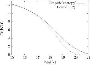
Accuracy of the bound on entropy
Concerning the bound on entropy given in 1, we checked our results on 8-round DES. For those simulations, we used a group of 76 linear approx-imations involving 13 key bits to perform a type 1 attack. The quality of the lower-bound (12) can be verified by estimating empirically the en-tropy. Figure 1 displays the empirical conditional entropy of K′ given Y for these equations as a function of log2(N), where N is the number of available plaintext-ciphertext pairs. There is an excellent agreement between the lower bound and the empirical entropies up to when we ap-proach the critical value ofN for which the lower bound is equal to zero. This kind of lower bound is really suited to the case when the amount of plaintext/ciphertext pairs is some order of magnitude below this critical value. This is typically the case when we want to decrease the amount of data needed at the expense of keeping a list of possible candidates forK′.
0 2 4 6 8 10 12
15 16 17 18 19 20 21
H
(
K
′|Y
)
log2(N)
Empiric entropy Bound (12)
Fig. 1.comparison between lower bound and empirical value of entropy.
A realistic type 1 attack on the full 16-round DES
Our aim in this experiment was to confirm that most of the time the right value of K′ = (< κi,K>)1≤i≤nbelongs to the list of 2H(K
′|Y)
trans-form. Generating the list and sorting it are thus two operations with the same complexity O(d2d) where d is the dimension of the space spanned by κ’s. This implies that to speed up the analysis phase, we have to use approximations that lead to a smalld. In the case when the set of approxi-mations does not have any structure, the analysis phase can be efficiently performed using a general decoding algorithm for random linear codes such as for instance the stochastic resonance decoding algorithm from Valembois [23]. There is still no proof of its complexity but it is quite simple to implement and actually efficient. The study of this decoding algorithm is out of the scope of this article but is a nice subject we wish to work on.
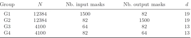
Using a Branch & Bound Algorithm, we found 74086 linear approxi-mations on the 16-round DES with biases higher than 2−28.84 (the biases are obtained by using the piling-up lemma). The space spanned by these
κ’s turned out to be 56. This is too much to use directly the fast Walsh-Hadamard transform. We choose to consider a subset of these approxi-mations (32968 out of 74086 spanning a vector space of dimension 42) which can be divided in 4 groups, each of them consisting of key masks
κi spanning a vector space of small dimensiond. We sum-up information
about these groups in Figure 2.
Group N Nb. input masks Nb. output masks d
G1 12384 1500 82 19
G2 12384 82 1500 19
G3 4100 64 82 13
G4 4100 82 64 13
Fig. 2.characteristics of the groups of approximations.
The numberN of available pairs was chosen to be small enough so that we can generate the data and perform the distillation phase in reasonable time. On the other hand, if we want our experiments to be relevant, we must get at least 1 bit of information about the key. These considerations lead us to chooseN = 239for which we get 2 bit of information out of 42 on the subkey.
We performed the attack 18 times. This attack recovers 42 bits of the key. For 239 pairs, the information on the key is of 2 bits. The entropy on the key is thus 40 bits. Our theoretical work suggests to take a list of size 2H(K′|Y)
= 240 to have a good success probability. Our experiments corroborate this. The worst rank over the 18 experiments is 240.88 and the rank exceeded 240in only 3 experiments out of 18. The (ordered) list of ranks for the 18 experiments is:
231.34,233.39,234.65,235.24,236.56,237.32,237.99,238.11,238.52,238.97,
239.04,239.19,239.27,239.53,239.85,240.28,240.82,240.88.
Comparison with Matsui’s attack:
The attack from [2] uses two approximations on 14-round DES with biases 1.19.2−21 in a type 3 attack. This kind of attack uses approximations with much better biases than a type 1 attack because they involve only 14 rounds instead of the full 16 rounds.
Despite this fact, we show here that the gap between 14-round ap-proximations and 16-round apap-proximations can be filled by using many approximations in type 1 attack. We demonstrate here that for a rather large range of number of plaintext/ciphertext pairs N, a type 1 attack has a better complexity than the best version Matsui’s type 3 attack [15]. This is first time that such a result is shown on the full DES.
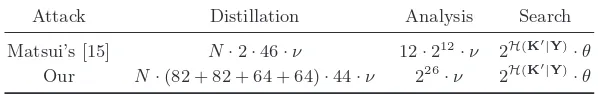
Figure 3 gives the formulas used to compute the complexity of the two attacks. Due to space constraints, we do not detail how we obtained the distillation and analysis phase complexities but they are essentially a direct application of the tricks of [24] and the work of [19]. We denote byν
theXORoperation complexity andθthe DES enciphering complexity (in-cluding key schedule). From the same amount of data, our attack obtains
Attack Distillation Analysis Search
Matsui’s [15] N·2·46·ν 12·212·ν 2H(K′|Y)
·θ
Our N·(82 + 82 + 64 + 64)·44·ν 226·ν 2H(K′|Y)
·θ
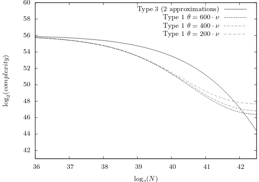
more information on the key. It improves the final search complexity at the cost of increasing the distillation phase complexity. To measure the gain of using a type 1 attack, we have to estimate the ratio ν/θ. The lower this ratio is, the more we gain using multilinear type 1 attack. For a standard implementation, 600·ν is a good estimate ofθ. We computed the complexities of the two attacks in terms of DES evaluations (θ) and plotted it as functions of the number of pairs in Figure 4. We restrict the plot to the value of N where type 1 attack competes with type 3 and we can see that this attack is better forN less than 242. We also plotted the complexities of the type attack for θ = 400·ν and θ = 200·ν to show that type 1 attack still competes with type 3 whenever enciphering is very efficient. Notice that with these estimates ofθ the complexity for Matsui’s attack remains the same as long as N is less than 242.5.
42 44 46 48 50 52 54 56 58 60
36 37 38 39 40 41 42
log
2
(
co
m
pl
ex
it
y
)
log2(N)
Type 3 (2 approximations) Type 1θ= 600·ν
Type 1θ= 400·ν
Type 1θ= 200·ν
Fig. 4.complexities of Matsui’s type 3 attack and our type 1 attack in terms of DES evaluations.
Remark on Matsui’s attack complexity:
mean. This observation, together with the complexity of computing mul-tidimensional probability laws in a general case, may confirm the interest of the approach presented in this paper.
5 Conclusion and further work
We have presented here a rather general technique in Lemma 1 to derive a sharp lower bound on the entropy of a key given (independent) statistics. We have applied it here to various linear cryptanalytic attacks, but the scope of this tool is much broader and it would be interesting to apply it for other classes of statistical attacks.
We performed a realistic type 1 attack on full 16-round DES using 32968 approximations and 239 plaintext/ciphertext pairs that confirmed our theoretical results.
Moreover, theoretical results predict that for 241pairs, the DES can be broken with high probability with complexity close to 248 while Matsui’s attack 2 needs 251.9 DES computations.
This work entails some further research interests.
It would be interesting to compare our theoretical results with some others [11, 25] for some particular type 3 attack.
Another interesting thing would be to perform a type 1 attack on another cipher (SERPENT for instance) to see if, for recent ciphers, type 1 attacks still can compete type 3 attacks.
A deep study of different decoding algorithms for the analysis phase is necessary as much as a precise complexity analysis of distillation phase complexity for type 1 attack (maybe using ideas from [19]).
References
1. Matsui, M.: Linear Cryptanalysis Method for DES Cipher. In: EUROCRYPT’93. Volume 765 of LNCS., Springer–Verlag (1993) 386–397
2. Matsui, M.: The First Experimental Cryptanalysis of the Data Encryption Stan-dard. In: CRYPTO’94. Volume 839 of LNCS., Springer–Verlag (1994) 1–11 3. Tardy-Corfdir, A., Gilbert, H.: A Known Plaintext Attack of FEAL-4 and FEAL-6.
In: CRYPTO’91. Volume 576 of LNCS., Springer–Verlag (1992) 172–181
4. Matsui, M., Yamagishi, A.: A New Method for Known Plaintext Attack of FEAL Cipher. In: EUROCRYPT’92. Volume 658 of LNCS., Springer–Verlag (1993) 81–91 5. Ohta, K., Aoki, K.: Linear Cryptanalysis of the Fast Data Encipherment
Algo-rithm. In: CRYPTO’94. Volume 839 of LNCS., Springer–Verlag (1994) 12–16 6. Tokita, T., Sorimachi, T., Matsui, M.: Linear Cryptanalysis of LOKI and s2DES.
7. Murphy, S., Piper, F., Walker, M., Wild, P.: Likelihood Estimation for Block Cipher Keys. Technical report, Information Security Group, University of London, England (1995)
8. Vaudenay, S.: An Experiment on DES Statistical Cryptanalysis. In: CCS 1996, ACM (1996) 139–147
9. Junod, P., Vaudenay, S.: Optimal key ranking procedures in a statistical crypt-analysis. In: FSE 2003. Volume 2887 of LNCS., Springer–Verlag (2003) 235–246 10. Kaliski, B.S., Robshaw, M.J.B.: Linear Cryptanalysis Using Multiple
Approxima-tions. In: CRYPTO’94. Volume 839 of LNCS., Springer–Verlag (1994) 26–39 11. Biryukov, A., Canni`ere, C.D., Quisquater, M.: On Multiple Linear
Approxima-tions. In: CRYPTO’04. Volume 3152 of LNCS., Springer–Verlag (2004) 1–22 12. Collard, B., Standaert, F.X., Quisquater, J.J.: Improved and Multiple Linear
Cryptanalysis of Reduced Round Serpent. In: Inscrypt 2007. Volume 4990 of LNCS., Springer–Verlag (2007) 51–65
13. Collard, B., Standaert, F.X., Quisquater, J.J.: Experiments on the Multiple Linear Cryptanalysis of Reduced Round Serpent. In: FSE 2008. Volume 5086 of LNCS., Springer–Verlag (2008) 382–397
14. Hermelin, M., Cho, J.Y., Nyberg, K.: Multidimensional Linear Cryptanalysis of Reduced Round Serpent. In: ACISP 2008. Volume 5107 of LNCS., Springer–Verlag (2008) 203–215
15. Junod, P.: On the Complexity of Matsui’s Attack. In: SAC 2001. Volume 2259 of LNCS., Springer–Verlag (2001)
16. Sel¸cuk, A.: On Probability of Success in Linear and Differential Cryptanalysis. J. Cryptol.21(2008) 131–147
17. Murphy, S.: The Independence of Linear Approximations in Symmetric Cryptol-ogy. IEEE Transactions on Information Theory52(2006) 5510–5518
18. Cover, T., Thomas, J.: Information theory. Wiley series in communications. Wiley (1991)
19. Collard, B., Standaert, F.X., Quisquater, J.J.: Improving the Time Complexity of Matsui’s Linear Cryptanalysis. In: ICISC 2007. Volume 4817 of LNCS., Springer– Verlag (2007) 77–88
20. Richardson, T., Urbanke, R.: Modern coding theory (2008)
21. Feller, W.: An introduction to probability theory and its applications. 3rd edn. Volume 1. John Wiley and Sons Inc., New York (1968)
22. Fourquet, R., Loidreau, P., Tavernier, C.: Finding Good Linear Approximations of Block Ciphers and its Application to Cryptanalysis of Reduced Round DES. In: WCC 2009. (2009) 501–515
23. Valembois, A.: D´etection, Reconnaissance et D´ecodage des Codes Lin´eaires Bi-naires. PhD thesis, Universit´e de Limoges (2000)
24. Biham, E., Dunkelman, O., Keller, N.: Linear Cryptanalysis of Reduced Round Serpent. In: FSE 2001. Volume 2355 of LNCS., Springer–Verlag (2001) 219–238 25. Hermelin, M., Cho, J.Y., Nyberg, K.: Multidimensional Extension of Matsui’s
Algorithm 2. In: FSE 2009. LNCS, Springer–Verlag (2009)
A Proofs
A.1 Proof of Lemma 1
H(Y|K′). From this we deduce that
I(K′;Y) = H(Y)− H(Y|K′)
= H(Y1, . . . , Yn)− H(Y1, . . . , Yn|K′). (15)
Here Equation (15) is a consequence of the fact that the a priori distri-bution over K′ is the uniform distribution and the entropy of a discrete random variable which is uniformly distributed is obviously nothing but the logarithm of the number of values it can take. Moreover (see [18, Theorem 2.6.6])
H(Y1, . . . , Yn)≤ H(Y1) +· · ·+H(Yn). (16)
On the other hand, by the chain rule for entropy [18, Theorem 2.5.1]:
H(Y1, . . . , Yn|K′) =H(Y1|K′) +H(Y2|Y1,K′) +· · ·+H(Yn|Y1, Y2, . . . , Yn−1,K′). (17) We notice now that H(Yi|K′, Y1. . . Yi−1) can be written as
P
k
R
Ri−1H(Yi|K′=k,Y1=y1,...,Yi−1=yi−1)f(y1,...,yi−1|K′=k)Pr(K′=k)dy1...dyi−1,
(18) where the sum is taken over all possible values k of K′ and
f(y1, . . . , yi−1|K′ = k)Pr(K′ = k) is the density of the distribu-tion of the vector (Y1, . . . , Yi−1) given the value k of K′ at the point (y1, . . . , yi−1). From conditional independence assumption (9) we deduce
thatH(Yi|K′ = k, Y1=y1, . . . , Yi−1=yi−1) =H(Yi|Ki′). By summing in
Expression (18) over y1, . . . , yi−1 and all possible values of
K′
1, . . . , Ki′−1, Ki′+1, . . . , Kn′ we obtain that
H(Yi|K′, Y1, . . . , Yi−1) = 1
2H(Yi|K
′ i= 0) +
1 2H(Yi|K
′
i= 1) =H(Yi|Ki′=ki) (19) Plugging in this last expression in Expression (17) we obtain that
H(Y1, . . . , Yn|K1′, . . . , Kn′) =H(Y1|K1′) +· · ·+H(Yn|Kn′). (20)
Using this last equation and Inequality (16) in (15) we finally deduce that
I(K′;Y) ≤ H(Y1) +· · ·+H(Yn)− H(Y1|K1′)− · · · − H(Yn|Kn′)
≤ n
X
i=1
H(Yi)− H(Yi|Ki′)≤ n
X
i=1
I(Ki′;Yi). (21)
A.2 Proof of Theorem 1
The proof of this theorem follows closely standard proofs of the direct part of Shannon’s channel capacity theorem [18], however most of the proofs given for this theorem are asymptotic in nature and are not suited to our case. There are proofs which are not asymptotic, but they are tailored for the case where all the σi’s are equal and are rather involved. We prefer
to follow a slightly different path here. The first argument we will use is an explicit form of the joint AEP (Asymptotic Equipartition Property) theorem.
For this purpose, we denote by (X,Y) a couple of random variables where X = (Xi)1≤i≤n is uniformly distributed over {0,1}n and Y =
(Yi)1≤i≤n is the output of the Gaussian channel described in Section 2
when X is sent through it. This means that
Yi= (−1)Xi+Ni, (22)
where the Ni are independent centered normal variables of variance σ2i.
Let us first bring in the following definition.
Definition 1. For ǫ > 0, we define the set Tǫ of ǫ-jointly typical
se-quences of {0,1}n×Rn by T ǫ
def
= S
x∈{0,1}n{x} ×Tǫ(x) with
Tǫ(x)
def
= {y∈Rn:|−log2(f(y))− H(Y)|< nǫ (23) ¯
¯−log2 ¡
f(y|x)2−n¢
− H(X,Y)¯¯< nǫ ª
(24)
where f(y) is the density distribution of Y and f(y|x) is the density distribution of Y given that X is equal tox.
The entropies ofY and (X,Y) are given by the following expressions Lemma 3.
H(Y) =
n
X
i=1
Cap(σ2i) +1
2log2(2πeσ 2
i)
H(X,Y) = n+
n
X
i=1 1
2log2(2πeσ 2
i)
Proof. Notice that with our model theYi’s are independent. Therefore H(Y) = Pn
i=1H(Yi). Moreover, by the very definitions of entropy and
mutual information: H(Yi) =H(Yi|Xi) +I(Xi;Yi); Xi is uniformly
Gaussian channel and the fact that the capacity attains its maximum for a binary input which is uniformly distributed we haveI(Xi;Yi) =Cap(σi2).
On the other hand H(Yi|Xi) is obviously the same asH(Ni). The
calcu-lation of this entropy is standard (see [18]) and gives
H(Ni) =
1
2log2(2πeσ 2
i) (25)
By putting all these facts together we obtain the expression for H(Y). Concerning the other entropy, with similar arguments we obtain
H(X,Y) = H(X) +H(Y|X)
= n+ X
x∈{0,1}n 1
2nH(Y|X=x)
= n+ X
x∈{0,1}n 1
2nH(N1, . . . , Nn)
= n+
n
X
i=1 1
2log2(2πeσ 2
i)
“Tǫ” stands for “typical set” since it is highly unlikely that (X,Y)
does not belong toTǫ:
Lemma 4. There exists a constant A such that
Pr((X,Y)∈/Tǫ)≤
A ǫ2n.
Before giving the proof of this lemma we will first give an interpreta-tion of entropy which provides an explanainterpreta-tion of why the probability of falling outside the typical set becomes smaller asnincreases.
Lemma 5. Let Ui
def
= −log2fi(Yi) where fi is given by
fi(y)
def
= 1
2q2πσ2
i
Ã
e−
(y−1)2 2σ2i +e−
(y+1)2 2σi2
!
We also denote by Vi
def
= −log2³gi(Yi−(−1)Xi) 2
´
where gi is the density
distribution of a centered Gaussian variable of variance σi2.
−log2(f(Y))− H(Y) =
n
X
i=1
Ui−E
à n X
i=1
Ui
!
−log2(f(Y|X)2−n)− H(X,Y) =
n
X
i=1
Vi−E
à n X
i=1
Vi
!
Proof. For the first equation we just have to notice that
−log2(f(Y)) =−log2(Πin=1fi(Yi)) =− n
X
i=1
log2(fi(Yi)) = n
X
i=1
Ui
and thatH(Y) =E(−log2f(Y)), which follows directly from the defini-tion of the entropy given in (5). The second equadefini-tion can be obtained in a similar way.
This implies that in order to estimate the probability that a point falls outside the typical set we have to estimate the probability that the deviation between a sum of n independent random variables and its ex-pectation is at least of order ǫn. In our case, it can be proven that for fixed ǫ, this probability is exponentially small in n. However, we prefer to give a much weaker statement which is also easier to prove and which uses only Chebyschev’s inequality, which we recall here
Lemma 6. Consider a real random variableX of variance var(X). We have for any t >0:
Pr(|X−E(X)| ≥t)≤ var(X)
t2 . (26)
To use this inequality we have to estimate the variances of the Ui’s
and theVi’s. It can be checked that
Lemma 7. There exists a constant A such that for any i we have
var(Vi)≤A and var(Ui)≤A.
Proof. Let us prove the first statement. Recall that from (22), we have
Ni = Yi − (−1)Xi.
¯
Vi def= Vi−E(Vi) = −log2 µ
gi(Ni)
2 
−E
µ
−log2 µ
gi(Ni)
2 ¶¶
=−log2(gi(Ni))−1
2log2(2eπσ 2
where the last equation follows from Expression (25). Hence:
¯
Vi= log2(e)
Ni2
2σ2i +
1
2log2(2πσ 2
i)−
1
2log2(2eπσ 2
i) =
log2(e) 2
µ
Ni2 σi2 −1
,
and therefore
var(Vi)def= E
h ¯
Vi2
i
= log2(e) 2 4 Z ∞ −∞ 1 q
2πσ2i
µ
u2
σi2 −1
¶2
e−
u2 2σ2
idu
= log2(e) 2 4 Z ∞ −∞ 1 √ 2π ¡
v2−1¢2
e−v
2 2 dv
where the last equation follows by the change of variable v = σu
i in the integral. This shows that the variance of Vi is constant. For the second
statement we will make use of the following inequalities. For nonnegative
u we have
e−
(u−1)2
2σi2 /2q2πσ2
i ≤fi(u)≤e −(u−1)2
2σ2i /q2πσ2
i. (27)
Recall that E(Ui) = H(Yi) = H(Yi|Xi) +I(Xi;Yi) =H(Ni) +I(Xi;Yi).
Note that 0 ≤ inf(Xi;Yi) ≤ H(Xi) = 1 by the properties of mutual
information (see [18][chapter 2]). And since H(Ni) = 12log2(2eπσi2) we
deduce that 1
2log2(2eπσ 2
i)≤E(Ui)≤
1
2log2(2eπσ 2
i) + 1. (28)
To simplify the expressions below we letu=Yi. Assume thatUi is greater
that its expectation and that this expectation is nonnegative. This means that −log2fi(u)≥E(Ui)≥0. We notice that
¯
Ui2 = (Ui−E(Ui))2
= (−log2(fi(u))−E(Ui))2
≤
µ
log2(e)(u−1) 2
2σ2
i
+ 1 +1
2log2(2πσ 2
i)−
1
2log2(2eπσ 2
i)
¶2
= µ
log2(e)(u−1) 2
2σ2
i
−1
2log2(e/2) ¶2
(29)
by using inequations (27) and (28). Let us now write
var(Ui) =E( ¯Ui)2 =
Z ∞
−∞
¯
Ui2fi(u)du
= Z 0
−∞
¯
Ui2fi(u)du+
Z E(Ui)
0 ¯
Ui2fi(u)du+
Z ∞
E(Ui) ¯
From the previous upper-bound on ¯Ui2 we deduce that
Z ∞
E(Ui)
¯
Ui 2
fi(u)du ≤ Z ∞
E(Ui)
„
log2(e)(u−1)
2
2σ2 i
−1
2log2(e/2)
«2 fi(u)du
≤
Z ∞
E(Ui)
„
log2(e)(u−1)
2
2σ2 i
−1
2log2(e/2)
«2 e−
(u−1)2 2σ2
i
p
2πσ2 i
du (30)
=
Z ∞
E(Ui)−1
σi
„
log2(e) v2
2 − 1
2log2(e/2)
«2 e−v
2 2
√
2πdv (31)
≤
Z ∞
−∞ „
log2(e)v
2
2 − 1
2log2(e/2) «2
e−v2 2
√ 2πdv,
where Inequality (30) is a consequence of (27) and Equality (31) follows from the change of variable v= uσ−1
i . The two other integrals in (29) can be treated similarly where instead of using (27) we use for negative values
ofu:e−
(u+1)2
2σi2 /2q2πσ2
i ≤fi(u)≤e −(u+1)2
2σ2i /q2πσ2
i. This yields a constant
upper-bound for all variances var(Ui).
We are ready now to prove Lemma 4:
Proof. We start the proof by writing
Pr((X,Y)∈/Tǫ) =Pr({|−log2(f(Y))−H(Y)|≥nǫ}∪{|−log2(f(Y|X)2−n)−H(X,Y)|≥nǫ}
≤Pr(|−log2(f(Y))−H(Y)|≥nǫ)+Pr(|−log2(f(Y|X)2−n)−H(X,Y)|≥nǫ) =Pr(|U−E(U)|≥nǫ)+Pr(|V−E(V)|≥nǫ)
withU def= Pn
i=1Ui andV def= Pni=1Vi. We use now Chebyschev’s
inequal-ity (Lemma 26) together with the upper-bounds var(U) =Pn
i=1var(Ui)≤
nA and var(V) =Pn
i=1var(Vi) ≤nA to obtain Pr((X,Y)∈/ Tǫ)≤ nǫ2A2.
Moreover, not only is it unlikely that (X,Y) does not fall inTǫ, but
the Euclidean volume (which we denote by “Vol”) of this set is not too large:
Lemma 8.
X
x∈{0,1}n
Vol(Tǫ(x))≤2H(X,Y)+ǫn
Proof. Let us notice that
1 = X
x∈{0,1}n 1 2n
Z
Rn
f(y|x)dy ≥ X x∈{0,1}n
1 2n
Z
Tǫ(x)
f(y|x)dy
≥ X
x∈{0,1}n
where the last inequality follows from (24) We will use this result to show that
Proposition 1. If ( ˜X,Y˜) is a couple of independent random variables, where X˜ is uniformly distributed andY˜ has the same distribution as Y, then Pr
³
( ˜X,Y˜)∈Tǫ
´
≤2−C+2nǫ with Cdef= Pn
i=1Cap(σi2).
Proof. We evaluatePr³( ˜X,Y˜)∈Tǫ
´
as follows
Pr(( ˜X,Y˜)∈Tǫ)=Px∈{0,1}n21n R
Tx(ǫ)f(y)≤ P
x∈{0,1}n21nVol(Tx(ǫ))2−H(Y)+ǫn
The last inequality follows from (23) in the definition of the typical set. We use now Lemma 8 to obtain
Pr³( ˜X,Y˜)∈Tǫ
´
≤ 1
2n2
H(X,Y)+ǫn2−H(Y)+ǫn≤2−n+H(X;Y)−H(Y)+2ǫn
By using the expressions for H(X,Y) and H(Y) given in Lemma 3 we deduce−n+H(X,Y)−H(Y) =−Pn
i=1Cap(σ2i).This finishes the proof.
These results can be used to analyze the following typical set decoder, which takes as inputs a vectoryinRnwhich is the output of the Gaussian channel described in Section 2 and a real parameterǫ, and outputs either “Failure” or a possible key ˜K∈ {0,1}n.
Typical set decoder(y, ǫ)
1 counter←0
2 for all possible valuesk of ˜K 3 do if y∈Tk(ǫ)
4 then counter←counter+ 1
5 result←k
6 if counter = 1
7 then return result
8 else return f ailure
This algorithm is therefore successful if and only ifyis in the typical set of the right key and if there is no other value k for ˜K for which y belongs to the typical set associated tok. Let us now finish the proof of Theorem 1.
Proof. Letk be right value of ˜Kand letC be the set of possible values of ˜K. The probabilityPerrthat the typical decoder fails is clearly upper-bounded by
Perr≤Pry,C(Tk(ǫ)) + X
k′∈C,k′6=k
whereTk(ǫ) denotes the complementary set ofTk(ǫ). On the one hand
Pry,C(Tk(ǫ)) =Pr((X,Y)∈/ Tǫ)≤
A ǫ2n.
by Lemma 4, and on the other hand for k′ 6=k:
X
k′∈C,k′6=k
Pry,C(Tk′(ǫ)) ≤ X
k′∈C
Pry,C(Tk′(ǫ)) = 2rPr ³
( ˜X,Y˜)∈Tǫ
´
≤ 2r−Pni=1Cap(σi2)+2ǫn
by Proposition 1. By plugging in these two upper bounds in the union bound (32) we obtain Perr≤ ǫA2n+ 2r−
Pn
i=1Cap(σi2)+2ǫn≤ A
ǫ2n+ 2−δn+2ǫn. We finish the proof by choosingǫ= 4δ.
B How to combine information from the 4 groups
Let us recall the problematic. Four groups of approximations are used to recover 42 bits of the master key. The two first groups (namely G1 and G2) involve 19 bits of the key each and the two others (G3 and G4) involve only 13 key bits. Some bits are common to some groups what explains that the overall set of approximations only involves 42 bits. We denote by LGi (1≤ i ≤ 4) the list sorted obtained after perfoming the Walsh Hadamard transformation on groupGi. Elements inLGi are of the form (k, li(k)) wherek∈F219/13 is the 13/19 bits candidate andli(k) the
log-likelihood of this candidate regarding theith group of approximations. The question is how do we combine the information obtained by the 4 groups of approximations to efficiently recover the rank of the good subkey in the sorted list of candidates.
First of all, notice that the log-likelihood of a subkey is the sum of the log-likelihoods obtained with each group of approximations that is
l(k) =l1(k) +l2(k) +l3(k) +l4(k).
The second thing to notice is that in our simulations, we know the value of the good key k∗. Thus, we can computel(k∗) from theLi’s.
We actually merge information from groups G1 and G3 (resp. G2 and G4) into 2 sorted lists L1 and L2. Since 6 bits are in common for each couple of groups, the size of these two lists is 226.
L1={(k1||k3, l1(k1) +l3(k3)),(k1, l(k1))∈LG1,(k3, l(k3))∈LG3}
L2={(k2||k4, l2(k2) +l4(k4)),(k2, l(k2))∈LG2,(k4, l(k4))∈LG4} Finally, subkeys from L1 and L2 have 10 common bits thus we split L2 into 210 subkey cosets L2,a of size 216 (with L2,a still sorted). Now, for
each subkey k∈L1, we have a listL2,k10 of all subkeys from L2 with the same common 10 bits ask. To compute the rank of the good subkey, we sum, for each subkey k∈L1, the number of subkeys in the subkey coset