Abstract
LIANG, AIHUA. Asymptotic Wave Solutions for Euler-Bernoulli and Timoshenko Beam by Ray Method and Stationary Phase Method. (Under the direction of Dr. F. G.
Yuan.)
The behavior of flexural (bending, transverse) waves in beam structures is of basic
importance in the stress wave theory and has been studied for many years. Many methods
have been attempted to understand the flexural waves in beams based on Euler-Bernoulli
and Timoshenko beam theories. Accurate numerical evaluations for transient waves in
structures are usually difficult due to the complexity of the governing equations.
The present research was aimed at developing asymptotic wave solutions that can
effectively describe one-dimensional flexural waves based on Euler-Bernoulli beam
theory and Timoshenko beam theory.
Two methods were introduced to obtain the asymptotic wave solutions for
Timoshenko and Euler-Bernoulli beams. One is stationary phase method, which derives
the asymptotic solution directly from the wave solution that can be expressed in terms of
the Fourier integral. From the features obtained from the stationary phase method, the ray
method is introduced to seek the asymptotic wave solutions from the governing equations
of wave motion. The asymptotic solutions obtained by the two methods, as expected, are
consistent, and the attributes of the wave motion are very clear to comprehend in the
asymptotic solutions. The amplitude function of the wave is composed of an arbitrary
decay rate proportional to t−1/2. The wave motion depends on one parameter t along the
ray x/t=cg.
The numerical calculations were then applied to initial-value problems,
boundary-value problems. The results show that the asymptotic solutions predict the transient wave
Asymptotic Wave Solutions for Euler-Bernoulli and Timoshenko
Beam by Ray Method and Stationary Phase Method
By
Aihua Liang
A thesis submitted to the Graduate Faculty of North Carolina State University
In partial fulfillment of the Requirements for the Degree of
Master of Science
Mechanical Engineering
Raleigh
2003
Biography
Aihua Liang was born in Huaian, Jiangsu Province, the People’s Republic of China
on October 2, 1970. She received her Bachelor degree in Engineering Mechanics from
Huazhong University of Science and Technology in 1995. She worked as a mechanical
engineer in Shanghai Scientific Instrument Factory, China Academy of Space
Technology from 1995 to 1999. She started her M.S. program of Mechanical Engineering
Acknowledgements
The author would like to express her appreciation to her committee chair, Dr. F. G.
Yuan, for his guidance, patience, and enthusiastic encouragement throughout the study
and work in the past two years.
The author also wishes to express her thanks to her committee members, Dr. M. N.
Noori and Dr. T. Zeng, for their kindness and valuable suggestions.
Sincere thanks go to Dr. S. Yang, who offered help in this research, especially in the
study of the ray asymptotic solutions for flexural waves.
The author would like to thank all the people from whom she has received help and
Table of Content
List of Figures... viii
1 Introduction... 1
1.1 Background of the Ray method ... 1
1.2 Flexural Waves in Structures ... 4
1.3 Asymptotic Wave Solutions for Beams... 6
2 Ray Theory... 9
2.1 Conventional Concept of rays... 9
2.2 Rays and Wave Fronts in Geometrical Optics... 10
2.2 Theory of Characteristics and Rays in First-order Partial Differential Equation .. 10
3 Flexural Wave Characteristics in Beams ... 17
3.1 Governing Equation for Timoshenko Beam and Euler-Bernoulli Beam... 18
3.2 Asymptotic Solution for One-dimensional Linear Dispersive Wave by Stationary Phase Method... 30
3.3 Asymptotic Expansion for Timoshenko Beam by Ray methods ... 39
3.3.1. Derivation of First-order PDE by Applying Asymptotic Expansion Series. 40 3.3.2. Determination along Rays... 43
3.3.3. Integration of the Amplitude Equation along Rays ... 45
3.4 Asymptotic Expansion for Euler-Bernoulli Beam by Ray methods... 47
3.5 Summary of General Asymptotic Solution for Timoshenko Beam and Euler-Bernoulli Beam ... 49
4 Numerical Results for Timoshenko and Euler-Bernoulli Beams ... 51
4.1.1. Exact Solutions of Initial-Value Problem for Euler-Bernoulli Beams ... 51
4.1.2. Asymptotic Solutions of Initial-Value Problem for Euler-Bernoulli Beams 54 4.1.3. Numerical Results... 56
4.2 Initial-Value Problem for Timoshenko Beams ... 61
4.2.1. Exact Solutions of Initial-Value Problem for Timoshenko Beams ... 61
4.2.2. Asymptotic Solution of Initial-Value Problem for Timoshenko Beam... 66
4.2.3. Numerical Results... 67
4.3 Boundary-Value Problem for Euler-Bernoulli Beams... 70
4.3.1. Exact Solutions of Boundary-Value Problem for Euler-Bernoulli Beams ... 70
4.3.2. Asymptotic Solutions of Boundary-Value Problem for Euler-Bernoulli Beams... 71
4.3.3. Numerical Results... 72
4.4 Boundary-Value Problem for Timoshenko Beams... 72
4.4.1. Exact Solutions of Boundary-Value Problem for Timoshenko Beams ... 72
4.4.2. Asymptotic Solutions of Boundary-Value Problem for Timoshenko Beams... 75
4.4.3 Numerical Results... 75
4.5 Comparison of Boundary-Value Problems of Euler-Bernoulli and Timoshenko Beam ... 76
5 Discussion and Conclusions ... 113
5.1 Conclusions... 113
List of Figures
Figure 2.1 Three types of rays………...9 Figure 2.2 Wave fronts of waves emitted by a point source and rays……….10 Figure 2.3 Solution surface for first-order PDE………..11 Figure 2.4 A solution surface for p= p(x,y) made up of characteristic curves…...13
Figure 2.5 Generation of the solution surface by characteristics...…...16 Figure 3.1 Timoshenko beam element subjected to load and its cross-section……..19 Figure 3.2 Path of the contour of integration……….35
Figure 4.1 Displacement response w/h versus time tc0/h at a fixed location x/h for Euler-Bernoulli beam with initial conditions:
0 ),
(
0
0 ∂ =
∂ =
= =
t
t t
w x
w δ ……….78
Figure 4.2 Displacement response along the ray x/t =cg for Euler-Bernoulli beam
with initial conditions: ( ), 0
0
0 ∂ =
∂ =
= =
t
t t
w x
w δ …...79
Figure 4.3 Displacement responses w/h versus time tc0/h at a fixed location x/h for Euler-Bernoulli beam with initial conditions:
0 ),
( ) (
0 0
0 ∂ =
∂ −
− =
= =
t
t t
w x
x H x H
w ..………...81
Figure 4.4 Displacement response along the ray x/t =cg for Euler-Bernoulli beam
with initial conditions: ( ) ( ), 0
0 0
0 ∂ =
∂ −
− =
= =
t
t t
w x
x H x H
w ………….84
Figure 4.5 Displacement response w/h versus tc0/h at a fixed location x/h for Euler-Bernoulli beam with initial conditions:
) ( ,
0
0
0 t x
w w
t
t ∂ =δ
∂ =
=
Figure 4.6 Displacement response along the ray x/t =cg for Euler-Bernoulli beam
with initial conditions: 0, ( )
0
0 t x
w w
t
t ∂ =δ
∂ =
=
= ……….89
Figure 4.7 Displacement response w/h versus time tc0/h at a fixed location x/h for Euler-Bernoulli beam with initial conditions:
) ( ) ( , 0 0 0
0 t H x H x x
w w
t
t ∂ = − −
∂ =
=
= ………..93
Figure 4.8 Displacement response along the ray x/t =cg for Euler-Bernoulli beam
with initial conditions: 0, ( ) ( 0)
0
0 t H x H x x
w w
t
t ∂ = − −
∂ =
=
= ………….97
Figure 4.9 Displacement response w/h versus time tc0/h at a fixed location
x
/
h
for Timoshenko beam with initial conditions: wt=0 =δ(x), 00 = ∂ ∂ = t t w , 0 0 = = t
ψ , 0
0 = ∂ ∂ = t t ψ ………..98
Figure 4.10 Displacement response along the ray x/t =cg for Timoshenko beam with
initial conditions: wt=0 =δ(x), 0
0 = ∂ ∂ = t t w
, ψ t=0 =0, 0
0 = ∂ ∂ = t t ψ ………...99
Figure 4.11 Displacement response w/h versus time tc0/h at a fixed location x/h for Timoshenko beam with initial conditions: wt=0=H(x)−H(x−x0),
0 0 = ∂ ∂ = t t w
, ψt=0=0, 0
0 = ∂ ∂ = t t ψ ………101
Figure 4.12 Displacement response along the ray x/t =cg for Timoshenko beam with
initial conditions: wt=0 =H(x)−H(x−x0), 0,
Figure 4.13 Displacement response w/h versus time tc0/h at a fixed location x/h for Timoshenko beam with initial conditions: wt=0 =0, ( )
0
x t
w
t δ
= ∂ ∂
=
,
0
0 =
= t
ψ , 0
0 = ∂ ∂
= t
t
ψ
………105
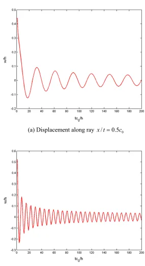
Figure 4.14 Displacement responses along the ray x/t=0.5c0 for Timoshenko beam with initial conditions: 0 , 0 ), ( , 0 0 0 0 0 ∂ = ∂ = = ∂ ∂ = = = = = t t t t t x t w w δ ψ ψ ………105
Figure 4.15 Infinite Euler-Bernoulli beam subject to sudden shear load……….71
Figure 4.16 Displacement response w/h versus time tc0/h at a fixed location x/h for Euler-Bernoulli beam with loading: Q(0,t)=Q0δ(t)δ(x)………….107
Figure 4.17 Displacement responses along the ray x/t =cg for Euler-Bernoulli beam with impact loading: Q(x,t)=Q0δ(x)δ(t)………...108
Figure 4.18 Displacement response w/h versus time tc0/h at a fixed location x/h for Timoshenko beam with impact loading: Q(x,t)=Q0δ(x)δ(t)……..110
Figure 4.19 Displacement responses along the ray x/t=0.5c0 for Timoshenko beam with impact loading: Q(x,t)=Q0δ(x)δ(t)………...110
Figure 4.20 Comparison of displacement responses w/h versus time tc0/h at a fixed location x/h between Euler-Bernoulli and Timoshenko beam with impact loading: )Q(x,t)=Q0δ(x)δ(t ………...112
Figure A-1 Group and phase velocity of a wave Packet………128
Figure A-2 Dispersive relations of beams………..134
Figure A-3 Phase velocity dispersion relation of beams………134
1 Introduction
1.1 Background of the Ray method
When people mention rays, naturally they think of light rays. Rays were originally
defined in optics as the paths along which the light travels. People with some common
sense of rays can do some small experiments of light rays by themselves, and they may
observe some very simple phenomena of light rays. For example, in a homogeneous
medium, a light ray propagating from one point to another is a straight line. When a ray is
incident upon a smooth surface with zero transmission coefficient, a reflected ray will be
produced. When a ray is incident upon the interface between one medium to another
different medium, a refracted ray will be generated. These phenomena may look very
simple today, but it is not so easy for ancient people to characterize these phenomena.
Euclid stated the first two phenomena, but he didn’t find a relation between the angle of
incidence and the angle of reflection. In about tenth century, Arabic scientist Alhazen
found that the angle of incidence was equal to the angle of reflection. In 1626, Snell
discovered that the angle of refraction angle was related to the angle of incidence by
some relations, the relation depended on the characteristic property of the medium. This
was the famous Snell’s law, which was published by Descartes in 1637. The theory that
light was a wave phenomenon was proposed by Huygens (1690) and then developed by
Newton (1704), Young (1802) and Freshel (1819). In the search for the correct equations
to describe light wave, various wave equations were proposed, and the wave equations of
In geometric optics, science of light, ray methods have been widely used to solve
optical wave phenomena. Basic geometrical optics is usually presented as a theory based
on the concepts of phase, rays and amplitude propagation along the rays (Anile et al.,
1993). Geometrical optics describes light wave’s propagation very successfully, this
prompted people to find the underlying ideas of wave motion in general as described by
linear PDE’s waves such as those in fluids, elastic media, etc. Until the second half of the
20th century, a systematic derivation of the laws of geometrical optics from the
fundamental equations of electromagnetism has been extensively carried out (Lunebourg,
1944; Kline and Kay, 1965; and Keller et al., 1956). Since then, some fundamental
advances about ray solution for linear PDE’s waves were made (Lax, 1957; Ludwig,
1966; and Friedlander, 1975).
Ray methods give us a natural synthesis of mathematical and physical insights into
wave propagation. In mathematics, ray methods are extensions to partial differential
equations of the well-known Wentzel-Kramers-Brillouin-Jeffreys (WKBJ) method for
ordinary differential equations. In physics, ray methods connect the basic concepts in
geometrical optics to a large class of phenomena. A lot of works have been done about
the numerical implementation of ray method in complex geometries and about the
extension of the method to the systems of equations of elastic and electromagnetic wave
propagation (Bleistein, 1984).
The wide use of numerical techniques in support of ray methods greatly enhances
their utilities. There is also a great practical advantage in applying numerical techniques
require the discretization on a spatial scale or temporal scale, which is a fraction of the
wavelength, thus it takes a long time to compute the numerical results, and it also
occupies a large space in the computer capacity. However, using ray method, if the
region of interest is far from the source of disturbance or for large values of t, the
discretization can be drastically reduced. Another advantage of using ray method is that
the ray method can reduce problems for partial differential equations (PDE) to the
solution of a system of first-order ordinary differential equations (ODE) that are linear in
the derivatives of the unknown constituents of the ray solution.
The wave motion is often governed by a high order partial differential equation,
which may be transformed to a first-order partial differential equation. This is known as
the eikonal equation whose solution can be interpreted in terms of wave fronts and rays
(Officer, 1958). The eikonal equation leads directly to the concept of rays. Wave
propagation may be described by successive wave fronts, and the normals to the wave
front define the direction of propagation are called rays (Lee, 1981). This concept is very
similar to that of conventional ray concept in geometrical optics.
Ray methods are not only applicable to linear wave motion, but also applicable to
nonlinear waves. Works about extending ray methods for linear wave equations to ray
methods for nonlinear wave equations were first done by Choquet (1969). These methods
use an asymptotic expansion, which has its origin in the WKBJ method. A lot of works
for applying ray methods to wave propagation have been done in various areas besides
electromagnetism. Some fundamental successes have been obtained in elasticity theory
(Hudson, 1980), fluid dynamics (Germain, 1977), plasma physics (Dougherty, 1970),
(BenMenahem and Singh, 1981; Hong and Helmberger, 1977; Richards, Witte and
Ekstrom, 1991), networks (Knessl and Tier, 1990), geophysics (Chapman, 1976), etc.
1.2 Flexural Waves in Structures
There have been strong interests in the behavior of flexural (bending) waves
propagating in structures. A structure can be as simple as a beam with a rectangular cross
section or a thin plate; it can be as complicated as the proposed space platforms that are
three-dimensional multi-member jointed grids with many attachments. It can also be
complicated like airplane fuselages and wings constructed as a combination of thin plates
and frame members (Doyle, 1997). The accurate evaluation of the flexural waves in
structures is usually very difficult due to the complexity of the governing equations
involved (Davies, 1953). In some cases, simplifying assumptions have to be introduced.
The behavior of flexural (bending) waves in beams provides basic transient wave
phenomena for more complicated structures. The simplest one-dimensional flexural
waves are based on Euler-Bernoulli beam theory, which only considers the lateral inertial
and elastic forces caused by bending deflections. Euler-Bernoulli beam theory is only
valid to predict the flexural waves for the cases of small wave numbers; because the
secondary effects such as shear deflections and rotary inertia have a negligible effect on
the first few modes of the beam (Kapur, 1966). The first and best known theory for
flexural waves, developed from the engineering standpoint, was given by Timoshenko
(Timoshenko, 1921 & 1922), who takes into account both the effect of rotation and the
The flexural waves in beams are governed by differential equations. It is possible to
solve the structural dynamics problems by starting with the partial differential equations
of motion and then integrating them. Many different methods have been attempted to
understand the flexural waves in beams based on Euler-Bernoulli beam and Timoshenko
beam theories. Laplace transform method was a popular one, a lot of work about the
solutions of the Timoshenko beam equations obtained by means of Laplace transform
have already done in the middle of 20th century (Uflyand, 1948; Dengler and Goland,
1952; Miklowitz, 1953). Boley and Chao (1955) derived the solutions of the Timoshenko
beam equations by the method of Laplace transformation for four types of loadings
applied to a semi-infinite beam. Numerical evaluations were also presented for two of
them by integrating the Laplace transforms along different integration paths for different
cases.
For flexural waves in thin plate structures, they are two-dimensional analogues of the
one-dimensional waves in beams. Thus, similar to beam theory, there are two
representative thin plate theories: classical plate theory and Mindlin (1951) plate theory.
Classical plate theory is based on two important assumptions, which are similar to that of
Euler-Bernoulli beams. First, the transverse normal stress may be neglected comparing to
the other stress components; second, according to Kirchhoff hypothesis, the linear
filaments of the plate initially perpendicular to the middle surface remain straight and
perpendicular to the deformed middle surface and suffer no extension (Graff, 1991).
Thus, both the rotary inertial and shear deformation are neglected in classical thin plate
theory. Although the simple governing equations of the classical thin plate theory can
When the frequency is high, the transverse shear effect should be taken into account.
Mindlin (1951) developed an approximate thin plate theory, which considers the effect of
transverse shear deformation. This can be considered as a generalization of the method
used in the development of Timoshenko beam theory.
Since the thin plate theory can be regarded as an extension of the beam theory,
solutions for the flexural waves in two-dimensional structures such as plate structures can
be solved by the similar methods used for the beams. The dispersion is very important in
the propagation for flexural waves in structures. More complicated structures will have
more complex dispersion relation, and it will be more difficult to characterize the
transient waves in the structures.
1.3 Asymptotic Wave Solutions for Beams
By understanding the complexity in the accurate evaluation of the flexural waves in
structures, it becomes necessary to find a simple way to describe the wave phenomena in
structures effectively. The goal of this project is to derive the asymptotic solutions for
flexural waves in beams and plates by stationary phase method and ray method.
Since ray is a conventional geometric optical concept, a simple introduction about
rays in geometric optics and in mathematics is given in Chapter 2. Geometric optics tells
us that the light wave phenomena consist of phase, wave front, ray, and amplitude. The
waves propagate along the rays in all directions, and different rays represent different
directions. In mathematics, the solutions for a hyperbolic partial differential equation may
equation are composed of the characteristic lines. The projections of the solution curves
on the argument plane are called rays.
In Chapter 3, two methods are introduced to derive the asymptotic wave solutions for
both Euler-Bernoulli and Timoshenko beams. One is the stationary phase method; the
other is the ray method. For dispersive waves in beams, the solutions can be written in a
Fourier style integral. The method of stationary phase can be used to derive the
asymptotic expansion for Fourier type integrals. The major contribution to the asymptotic
expansion of the integral can be determined by the immediate neighborhood of the
stationary phase points. Thus it is feasible to compute the integral around the stationary
phase points. The ray solutions are obtained by directly applying a proper asymptotic
series form to the governing equations of the beam, then collecting the terms with like
orders yields a system of first-order ordinary equations for the wave amplitude, wave
number and frequency respectively. By applying the dispersion relations of the beam, the
ray solution for the amplitude of the wave is found to be composed of two terms: one is
an arbitrary function which can be determined by initial and/or boundary conditions, the
other is a time decay rate proportional to t−1/2. Along a specific ray, the arbitrary function
will keep constant, and the solution of the amplitude will simply decay witht−1/2. It is
also found that the rays introduced in the amplitude equation and the equation of wave
number are the same. The phase, θ =kx−ωt, can be obtained by the wave frequency and the wave number. The comparison between the stationary phase solutions and the
asymptotic solutions are made at the end of the chapter, it can be found that these two
asymptotic solutions are consistent. A great advantage for the ray solution is that it can
In order to verify the asymptotic solutions derived in Chapter 3, numerical
computations are applied for both the exact solutions and the asymptotic solutions in
Chapter 4. The exact solutions are derived by directly taking the Fourier transform or
Laplace transform to the high order partial differential equations, then take the inverse
Fourier or Laplace transformation and apply the initial and/or boundary conditions to the
solution. Due to the complicated dispersion relations, the integrands in the exact solutions
are high oscillatory slow decay functions; Gauss-Legendre method (Yan, 1991; Davis
and Rabinowitz, 1967) is applied to obtain the integrations in this project. The numerical
plots for different initial conditions and/or boundary conditions are obtained for both
exact solution and asymptotic solution, and comparisons are made between them.
Summary about the numerical results for the exact solutions and the asymptotic solutions
are also made in this chapter.
There are some important advantages to use asymptotic wave solutions. First of all, it
can save much more time and capacity in the computer, especially for complicated
structures with higher order governing equations. Second, the contents of the flexural
waves are very clear in the formulas. From the numerical results, it is believed that we
2 Ray Theory
2.1 Conventional Concept of rays
Ray was originally defined in optics as the paths along which light travels, and they
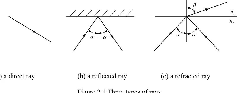
were widely used in geometric optics (Keller, 1978). There are three types of rays in
optics, direct rays, reflected rays and refracted rays, which are shown in Figure 2.1.
α α α
β
α
2
n
1
n
(a) a direct ray (b) a reflected ray (c) a refracted ray
Figure 2.1 Three types of rays
Figure 2.1 shows that a direct ray between two points in a homogeneous medium is a
straight line. A reflected ray will be generated when a ray is incident upon a smooth
surface with zero transmission coefficients, and the angle of reflection is equal to the
angle of incidence. When a ray is incident upon the interface between one medium to
another different medium, both reflection ray and refracted ray will be generated, the
reflection ray obeys the reflection law and the refraction ray obeys the Snell’s law, which
is:
2 1
sin sin
n n =
α β
Here ni, the index of refraction of medium i, is a characteristic property of medium i
(i=1,2). When the medium i is homogeneous, ni is constant.
2.2 Rays and Wave Fronts in Geometrical Optics
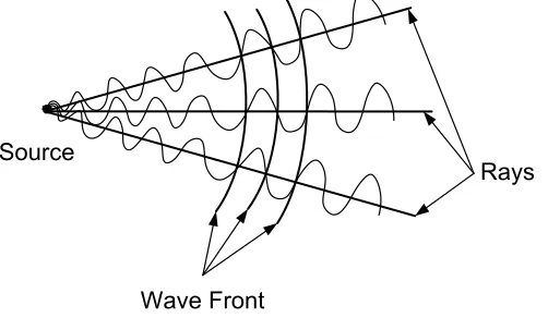
Geometrical optics describes light wave propagation very clearly (Fry, 1969). The
concept of a wave front can be developed by considering a disturbance starting from a
point source and spreading out as waves in all directions. The disturbance will reach
points equally distant from the source at the same time; the spherical surface, which is the
locus of these points, is called a wave front. Thus, wave propagation may thus be
described by successive wave fronts. A line perpendicular to a wave front represents the
direction of propagation of the wave front, and such line is called a ray (see Figure 2.2).
Figure 2.2 Wave fronts of waves emitted by a point source and rays
2.2 Theory of Characteristics and Rays in First-order Partial Differential
Equation
Partial differential equations are central to mathematics, whether in pure mathematics
or applied mathematics. They arise in mathematical models whose dependent variables
Source
Wave Front
Assuming that there is a function of two variables u(x,y), the solution for u(x,y)
can be expressed as a surface in three-dimensional space or a family of level curves in
two-dimensional space. Both representations will be proved very useful. A general
first-order partial differential equation (first-first-order PDE) governing u(x,y) can be simply
written in the form as:
0 ) , , , ,
(x y u p q =
F (2.2-1)
where ,p=ux q =uy. In order to ensure that the equation above is a truly partial
differential equation, it is required that
0 ≠ p
F and/or Fq ≠0 (2.2-2)
Assume that the solution for Eq. (2.2-1) is sufficiently smooth to allow the
interchange of orders of the differentiation, and then one can have
x
y q
p = (2.2-3)
The increments of u may be expressed as:
qdy pdx dy u dx u
du= x + y = + (2.2-4)
The equation above can be rewritten as:
0 ) 1 (− = +
+qdy du
pdx (2.2-5)
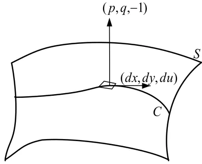
This equation states that the normal vector (p,q,−1) is perpendicular at each point to any
C
)
1
,
,
(
p
q
−
)
,
,
(
dx
dy
du
S
Figure 2.3 Solution surface for first-order PDE
S denotes the boundary conditions, and C represents the characteristic line in the figure above. In order to solve for the integration surface u(x,y) in Eq. (2.2-4), p and q
should be obtained first. Note that for a solution of Eq. (2.2-1), small increments in x and y produce no change in the value of F. That is,
y q F q F qF F
x p F p F pF F F
y q x p u y
y q x p u x
∆ +
+ + +
∆ +
+ + = ∆ =
) (
) (
0
(2.2-6)
Since the increments in x and y are independent, the coefficients in the equation above must be zero. Thus, one has:
u x y q x
pp F p F pF
F + =− − (2.2-7)
u y y q x
pq Fq F qF
F + =− − (2.2-8)
Considering the two equations above as two first-order partial differential equation for p
and q, then one can call them the governing equations for p and q. If Eq. (2.2-1) does
differential equations for p and q can be obtained. Similarly, one can write the
increments of p and q along their solution surfaces:
dy p dx p
dp= x + y (2.2-9)
dy q dx q
dq= x + y (2.2-10)
These two equations imply that the normal vector (px,py,−1) is perpendicular at each
point to any tangent vector (dx,dy,dp) to the solution surface of p; the normal vector
) 1 , ,
(qx qy − is perpendicular at each point to any tangent vector (dx,dy,dq) to the solution
surface of q.
Comparison of Eq. (2.2-9) with Eq. (2.2-7) suggests that one can view the solution
surface for p as being made up of a family of curves, on each of the curves, the direction
of the tangent of the curves at each point is given by (Fp,Fq,−Fx −pFu) which is the
same direction as (dx,dy,dp). These curves are called the characteristic curves (See
Figure 2.4). Thus, the solution surface for p is made up of characteristic curves on which
u x q
p F pF
dp F
dy F dx
+ − =
= (2.2-11)
When thinking of the solution p(x,y) as a family of level curves in the (x,y) plane,
the corresponding curves of interest are the projections of the characteristics onto the
Figure 2.4 A solution surface for p= p(x,y) made up of characteristic curves, each of which is
tangent to the vector with direction numbers (Fp,Fq,−Fx− pFu) at each point on the surface p
Similarly, one can express the solution q(x,y) as a family of characteristic curves as:
u y q
p F qF
dq F
dy F dx
+ − =
= (2.2-12)
Now it is found that the rays (or the base characteristics) for the governing equations for
p and q are the same, and the equations can be viewed as describing the simultaneous
propagation of p and q along the rays.
From Eqs. (2.2-4), (2.2-11) and (2.2-12), the change in ualong the same rays can be written as:
) / )( (pFp qFq dx Fp qdy
pdx
du= + = + (2.2-13)
Combining Eq. (2.2-13) with Eqs. (2.2-11) and (2.2-12), a complete set of equation is
given by:
qF F
dq pF
F dp qF
pF du F
dy F dx
+ − = + − = + =
The determination of u for each (x,y) on a ray defines a characteristic curve in three-dimensional space. Since one can also solve for p and q, then a solution of this
system of equations also yields a normal direction of the solution surface at each point on
the characteristic curve (see Figure 2.3).
In )(x,y,u space, a curve may be given by
= = =
) (
) (
) (
t u u
t y y
t x x
where t is a parameter, then one can rewrite the equation Eq. (2.2-14) in the form:
) (
) (
u y
u x
q p q p
qF F dt
dq
pF F dt
dp
qF pF dt du
F dt dy
F dt dx
+ − =
+ − =
+ = = =
(2.2-15)
By solving the ordinary differential equations above, the curve constructed lies in a
solution surface for all t. If initial boundary conditions at t=0 are set as: ),
(
0 s
x
x= y= y0(s) u=u0(s) (2.2-16)
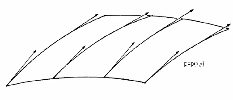
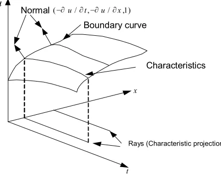
(Here, s represents a parameter for the boundary condition), then the solution surface also passes through the boundary curve. As s varies, the family of solution curves (also called characteristics) generates a surface, as shown in Figure 2.6, which is the required
as discussed before, the projections of the solution curves of Eq. (2.2-15) onto the (t,x)
plane are the rays.
t
u
x
Boundary curve Normal(−∂u/∂t,−∂u/∂x,1)
Characteristics
Rays (Characteristic projection)
Figure 2.5 Generation of the solution surface by characteristics
3 Flexural Wave Characteristics in Beams
The behavior of flexural (bending or transverse) waves in beams has been of interest
in thorough understanding basic transient wave propagation concepts and dispersion
phenomena that can be useful in analyzing waves in more complicated structures.
Different methods have been attempted to understand elastic waves based on
Euler-Bernoulli and Timoshenko beam theories. Solutions due to different types of transverse
impact loading for Bernoulli-Euler and Timoshenko beam equations were obtained by
means of the Laplace transform technique (Boley and Chao, 1955). A spectral method for
analyzing the wave phenomena in beams has been investigated by Doyle (1989). A lot of
work on long-time far-field solutions in beams has been examined by Miklowitz
(Miklowitz, 1978). A finite element model together with a state variable approach to
calculate the dynamic response of the beam under an impact was also recently studied
(Li, 2002).
In the first part of this chapter, Timoshenko beam theory is formulated, and then it is
reduced to classical Euler-Bernoulli beam theory by ignoring the rotary inertia and
transverse shear effect. Subsequently two methods are introduced to obtain the
asymptotic solutions for Timoshenko and Euler-Bernoulli beams. One is stationary phase
method; the stationary phase asymptotic solution is derived directly from the wave
solution in terms of the Fourier integral, which physically interprets the exact solution
form for linear dispersive waves in beams. The other method is a ray method. From the
features obtained from the stationary phase method, the ray method seeks asymptotic
asymptotic solution is obtained by solving the wave numbers, wave frequencies, and the
amplitude along the ray. Along the rays for each wave mode, the wave number and thus
frequency and group velocity remain constant. For each flexural wave mode, the slopes
of the rays are the group velocity. The amplitude function of the wave consists of two
parts; one is an arbitrary function, which can be determined by initial and/or boundary
conditions, the other is a time decay rate proportional to t−1/2. The comparison between
the ray asymptotic solution and the stationary phase asymptotic solution will be made at
the end of the chapter, and then more general asymptotic solution forms under initial
value and boundary value problems will be discussed.
3.1 Governing Equation for Timoshenko Beam and Euler-Bernoulli Beam
In deriving beam theories for slender beams, it is assumed that the neutral axis of the
cross section of the beam is a straight line and that the envelopes of the principal axes
through the neutral axis are two mutually perpendicular flat planes. Taking the x-axis in
the direction of the neutral axis and the y- and z-axes parallel to the principal directions,
the x-, y-, and z-axes form a right-handed Cartesian coordinate system (see Fig. 3.1).
dx
x
V
V
∂
∂
+
x
0
q
dx
x
M
M
∂
∂
+
M
V
dx
z
w
xz
γ
xz
γ
x w
∂ ∂ −
u
x
ψ
(b) Undeformed and deformed geometries for a Timoshenko beam element
Figure 3.1 Timoshenko beam element subjected to load and its cross-section
Since the longitudinal dimension of the slender beam is much larger than its lateral
dimensions, it is common in deriving the beam theory to employ the following
assumption. That is, the stress components σy, σz, and τyz may be neglected in
comparison with the other stress components.
0 = τ = σ =
σy z yz (3.1-1)
Then the constitutive relations for solids may be reduced to
xy xy
xz xz
x
x =Eε τ =Gγ τ =Gγ
σ , , (3.1-2)
For deriving the Euler-Bernoulli beam equation, two important kinematic
assumptions are made. First, the cross sections which are perpendicular to the neutral axis
before bending remain plane and perpendicular to the deformed neutral axis and thus no
shear strains in their planes. Second, the effects of rotary inertia are not taken into
account. In fact, the variation in shear stress across the cross section leads to the shear
deformation, which means the plane cross-section initially perpendicular to the neutral
Timoshenko beam theory (Graff, 1991), it is assumed that plane sections still remain
plane, but are not normal to the neutral plane. The equations of motion of the beam can
readily be derived by considering the equilibrium of shear force, bending moment, and
distributed transverse load shown in Fig. 3-1a. In the sign convention, the positive stress σx in the positive z-direction induces positive moment; the positive shear stress τxz in the
positive x-direction gives positive shear force. The transverse loading q0(x, t) is assumed
to vary arbitrarily with position and time. A parameter ψ is introduced to measure the
slope of the cross section due to effects of the bending. When considering both the rotary
inertia and the deflection due to the transverse shear, the slope of the transverse
displacement )w(x,t will depend not only on the rotation ψ(x,t) due to bending, but also
on the shear angle γxz(x,t). The deformed geometry for the Timoshenko beam element is
shown in Fig. 3-1b.
The following quantities can then be defined as:
w = transverse displacement of the neutral plane of the beam
z w
y ∂
∂ − =
θ = slope of the neutral plane of the beam
ψ = slope of the cross-section due to effects of the bending
xz
γ = shear angle
x w ∂ ∂ +
ψ = loss of slope, equal to the shear angle γxz
By confining the beam problem to small displacement theory, the displacements
) , ( ) , , ( 0 ) , , ( ) , ( ) , ( ) , , ( t x w t z x W t z x V t x z t x u t z x U = = + = ψ (3.1-3)
The non-vanishing strain components provided by Eq. (3.1-3) are:
ψ γ ψ ε + ∂ ∂ = ∂ ∂ + ∂ ∂ = ∂ ∂ = x w x z x u x U xz
x , (3.1-4)
Since the transverse shear strain is taken as a constant through the beam thickness, a
shear adjustment coefficient κ is introduced such that transverse shear force would be
equal to the actual shear force in magnitude, which is
κ γ γ
τ dA G dA (G A)
V xz
A xz
A xz = =
=
∫
∫
(3.1-5)where γxz is due to the shearing effect, which is taken as a constant through the thickness
of the beam. =
∫∫
AdydzA is the area of the cross section and V has a unit of force. The
value of κ depends on the shape of the cross section and the frequency of the vibration.
Mindlin (Mindlin, 1955) suggested that whenκ =π2 /12; the Timoshenko beam
equations give good results for both low and high frequencies of slender beams,
regardless of the end conditions. This parameter is usually designated as the Timoshenko
shear coefficient.
The assumption is made that the relation between bending moment and curvature still
holds, and then the bending moment of the cross section can be expressed as:
∫
∫
= = ∂∂=
A x
A xzdA E zdA EI x
M σ ε ψ (3.1-6)
where I z dydz A
∫∫
= 2 is the moment of inertia of the cross section and M has a unit of
Substituting the expression for γxzobtained from Eq. (3.1-4) into Eq. (3.1-5) yields + ∂ ∂ = κ ψ x w AG
V (3.1-7)
For the balance of the force in the vertical direction of the infinitesimal beam
element, by considering the inertia force intensity (force/length) 22 t
w A
∂ ∂
−ρ as a
distributed load intensity (force/length) q0(x, t) one can obtain
2 2 0 t w A q x V ∂ ∂ = + ∂ ∂ ρ (3.1-8)
where m=ρA, m is has a unit of mass per unit length along the beam, and ρ is the mass
per unit volume (mass density).
For the balance of the moment about y-axis passing through the neutral axis of the
element, one has
2 2 t I x M V ∂ ∂ = ∂ ∂ +
− ρ ψ (3.1-9)
where the right hand side of Eq. (3.1-9) represents the rotary inertia given by the product
of the mass moment of inertia of the cross section and the angular acceleration.
Substituting Eq. (3.1-6) and Eq. (3.1-7) into Eq. (3.1-8) and Eq. (3.1-9), the equations
of motion for Timoshenko beams are given by
2 2 2 2 2 2 0 2 2 t I x I E x w A G t w A q x w x GA ∂ ∂ = ∂ ∂ + + ∂ ∂ − ∂ ∂ = + ∂ ∂ + ∂ ∂ ψ ρ ψ ψ κ ρ ψ κ (3.1-10)
governing equations represent the physical coupling that occurs between them. One mode
of the deformation is simply the transverse deflection of the beam measured byw(x,t).
The other is the transverse shear deformationγxz, which is measured by +ψ ∂ ∂ x w
.
In some cases, it is convenient to reduce the two governing equations to a single
governing equation in terms of transverse displacement and the governing equation can
be reduced to that in classical Euler-Bernoulli beam theory. One can differentiate the
second equation in Eqs. (3.1-10) with respect tox,
2 3 3 3 2 2 t x I x I E x x w GA ∂ ∂ ∂ = ∂ ∂ + ∂ ∂ + ∂ ∂
− κ ψ ψ ρ ψ (3.1-11)
then re-arranging the first equation of Eqs. (3.1-10) gives
κ κ ρ ψ GA q t w G x w x 0 2 2 2 2 − ∂ ∂ + ∂ ∂ − = ∂ ∂ (3.1-12)
Substituting Eq. (3.1-12) into Eq. (3.1-11) leads finally to
2 0 2 2 0 2 0 4 4 2 2 2 2 2 4 4 4 1 t q GA I x q GA EI q t w G I t w A t x w G E I x w I E ∂ ∂ + ∂ ∂ − = ∂ ∂ + ∂ ∂ + ∂ ∂ ∂ + − ∂ ∂ κ ρ κ κ ρ ρ κ ρ (3.1-13)
This is a fourth-order differential equation in w for Timoshenko beam. While this form of
governing equation is more usual in deriving the dispersion relation and group velocity;
in general the governing equations (3.1-10) are more useful in obtaining wave modes and
the solutions for initial and boundary value problems.
If neglecting the rotary inertia, but still taking the shear deformation into account,
i.e., the right side of the second equation of (3.1-10) which is due to rotary inertia
2 0 2 0 2 2 2 2 4 4 4 x q GA EI q t w A t x w G EI x w I E ∂ ∂ − = ∂ ∂ + ∂ ∂ ∂ − ∂ ∂ κ ρ κ ρ (3.1-14)
If both the rotary inertia and shear deformation are neglected, i.e. setting G→∞in Eq. (3.1-14), then the governing equation of motion based on Timoshenko beam theory
reduces to that based on Bernoulli theory. Thus, the governing equation for
Euler-Bernoulli beams is given by
0 2 2 4 4 q t w A x w EI = ∂ ∂ + ∂ ∂ ρ (3.1-15) Phase velocity
A main characteristic of wave motion traveling in the medium is its velocity. In
principle, there exist two types of wave velocities, the phase velocity and the group
velocity. The first is the velocity of plane harmonic waves; while the second represents
the velocity of wave groups or wave packets.
Considering the plane (harmonic) wave solutions of the form
) ( 2 ) ( 1 , t kx i t kx
i B e
e B
w= −ω ψ = −ω (3.1-16)
In these relations, the quantity ω is the angular frequency or circular frequency of the
motion, it is measured in radians per unit of time, the cyclic frequency f, which is usually
referred to merely as the frequency of the motion, is given by
π ω 2 =
f (Hz), and its
reciprocal is called the period T,
f T = 2 = 1
ω π . λ π = 2
k is the wave number of wave
(radians/length or 1/length), i.e., the number of waves in 2π units of length. λ is the
considered as a spatial frequency, in analog with temporal frequency. The
correspondence between time and space variables are given by
T 2 Frequency
Period ω π
ω = T , λ π λ 2 Wavenumber Wavelength = k k
Substituting these solutions in Eqs. (3.1-16) into Eqs. (3.1-10) results in two
transcendental equations with transverse loading q0= 0,
0 ) ( 0 ) ( 2 2 2 1 2 1 2 2 = ω ρ − + κ + κ = κ + ω ρ − κ − B I EIk GA kB iGA kB iGA B A k GA (3.1.-17)
This is a set of two homogeneous equations in B1 and B2. In order to have a nontrivial
solution, the determinant of the coefficients of B1 and B2 must vanish. The resulting
equation is known as the dispersion equation
0 )
)(
(GAκk2−ρAω2 GAκ+EIk2 −ρIω2 −G2A2κ2k2 = (3.1-18)
or simplifying,
0
1 2 2 2 4
4 ω =
κ ρ + ω − ω κ + − ρ GA I k G E A I k A EI (3.1-19)
This equation expresses a relation between ω and k. Since ω is a function of the
wavelength ( k
π
λ = 2 ), the waves of the beam are dispersive. Using the identity ω=kcp,
the dispersion can be written in two alternate forms, which relates k and cp and ω and cp
respectively
0
1 4 2 2 2 4 4
4 − + =
+
− p p k cp
GA I c k c k G E A I k A EI κ ρ κ
ρ (3.1-20)
or
0
1 4 2 2 4 4 4
4 − + =
+
− p p cp
GA I c c G E A I A EI ω κ ρ ω ω κ ω
where cp is the phase velocity.
If one considers the equations of motion governed by the fourth-order differential
equation in w shown in Eq. (3.1-13), a plane wave solution is again assumed to be in the
form
) (kx t i Be
w= −ω (3.1-22)
and substituting Eq. (3.1-22) into Eq. (3.1-13) with q0 = 0 leads to the identical dispersion
relation as in Eq. (3.1-19).
In the following, the limiting behavior of Eq. (3.1-20) that relates cp and k is
investigated. In particular, consider the behavior for short wavelengths (k →∞). This can
be approached by factoring k4 from the equation and letting k → ∞. Then the equation
reduces to
0
1 2 + 4 =
+
− p cp
GA I c
G E A
I A EI
κ ρ κ
ρ (3.1-23)
or 4 1 2 + 2 =0
+ −
ρ κ κ
ρ
κ GE
c G
E G
cp p (3.1-24)
This equation has two roots:
ρ κ
G c
cp = 0, (3.1-25)
where
ρ
E
c0 = and the negative roots that represent waves propagation in the opposite
direction are ignored. These two limits are associated with two basic wave modes that are
To determine the cutoff frequencies, the wave number k approaching zero (long
wavelengths) for the dispersion relation that relates ω and k is considered. Taking the
limit of Eq. (3.1-19) as k→ 0, one has
0
4
2 + =
− ω
κ ρ ω
GA I
(3.1-26)
which has two roots
I GA
c ρ
κ
ω =0, (3.1-27)
Thus, one of the modes has a finite cutoff frequency. Further, as k = ε→ 0 the governing
equations (3.1-17) become
0 ) (
) (
0 ) (
2 2 1
2 1
2
= −
+
= +
B I GA B
iO
B iO B A
c c
ω ρ κ ε
ε ω
ρ
(3.1-28)
where O(ε) represents the value of order ε. As ωc→ 0, from the first equation of (3.1-28)
one has B1 ≠ 0, B2 = 0. In this case, the plane wave motion is given by
0 ,
1 =
=Be−iωct ψ
w (3.1-29)
This mode is associated with pure bending motion.
As ωc→
I GA
ρ κ
, from the second equation of Eq. (3.1-28) one has B2 ≠ 0, B1 = 0. For
the wave behavior, the plane wave motion is given by
0
=
w , ψ =B e−iωct
2 (3.1-30)
For Euler-Bernoulli theory, substituting the plane wave solution of Eq. (3.1-22) into
Eq. (3.1-15) with q0 = 0, the following dispersion relation can be obtained:
0
2
4 −ω =
ρAk EI
(3.1-31)
or
ω ρ
4 1
=
A I E
cp (3.1-32)
Clearly there is no cutoff frequency for the Euler-Bernoulli beam and as ω approaches
infinity, cp approaches without bound. This anomaly is the result of the assumptions
made in the Euler-Bernoulli theory. A refinement of the Euler-Bernoulli theory that does
not contain this deficiency is the Timoshenko theory. The detail is given in Appendix A
for dispersion behavior of Euler-Bernoulli and Timoshenko beams in terms of
non-dimensional parameters.
Group velocity
Although each of the plane waves seems to act independently, in dispersive media,
the idea of a definite velocity for the entire continuous propagating waves becomes
vague. The phenomenon of dispersion is then related to group velocity, defined as the
velocity which a wave packet is propagated. To illustrate the group velocity concept, one
considers a wave packet that arises from the interaction of two plane waves of unit
amplitude and slightly different wave numbers and frequencies. One may write
) cos(
) cos(
) ,
(x t kx t k1x 1t
where k and ω are the wave number and angular frequency of the first wave and
ω ∆ ω
ω1 = + , k1 =k+∆k. Using a trigonometric identify and neglecting higher-order terms and write Eq. (3.1-33) as
) cos(
2 cos 2 ) ,
( t kx t
k x t
x
w ω
∆ ω ∆ κ
∆ −
−
= (3.1-34)
Since ∆ω and ∆k are small, one can see that w is an amplitude-modulated wave with a slowly varying amplitude given by the first low frequency term of the above equation
(envelope). The amplitude-modulated wave is the envelope of the high-frequency wave
with frequency ∆ω traveling with the wave speed cp. The wave packet (envelope) has
the frequency ω1 =ω +∆ω travels with the group velocity cg. To obtain cg one considers
one cycle of the first factor. One thus sets
k t x
∆ ω ∆
= (3.1-35)
One then defines the group velocity cg as
dk d k
cg ω
∆ ω ∆
∆ =
= →0
lim (3.1-36)
The group velocity may be alternately represented in terms of cp and k or cp and the wave
length
k
π λ = 2 :
λ λ ω
d dc c
dk dc k c dk d
c p p
p
g = = + = − (3.1-37)
Another aspect of wave propagation which travels at the group velocity is the energy of
the plane wave trains. Consider Eq. (3.1-33)
) cos(
2 cos 2 ) ,
( t kx t
k x t
x
w ω
∆ ω ∆ κ
∆ −
−
Define the energy density as
) (
cos 2
cos
4 2 2 2 2
2
t kx t
k x k A
t w
E ω
∆ ω ∆ ∆
ρω
ρ −
− =
∂ ∂
= (3.1-39)
Taking the time average of this expression over several periods T, the average energy
density can be expressed as
−
≈ t
k x k A
Eav
∆ ω ∆ ∆
ρω
2 cos
2 2 2 2 (3.1-40)
This suggests that the rate of time-averaged energy density propagation is proportional to
the group velocity.
3.2 Asymptotic Solution for One-dimensional Linear Dispersive Wave by
Stationary Phase Method
After obtaining the governing equations for both Timoshenko and Euler-Bernoulli
beams, the general solutions for the flexural wave in the beam can be obtained by solving
the governing equations.
For one-dimensional linear dispersive waves, the elementary solutions can be
expressed in a form of sinusoidal wave trains (Whitham, 1974). Thus, the elementary
solution for the beams can be written in the form of plane wave:
) (
) ,
(x t Aeikx t
w = −ω (3.2-1)
where k is the wave number of the plane wave, ω is the angular frequency, Ais the amplitude. In the elementary solution, k, ω, and A are arbitrary constants. The linearity
equations are linear, A factors out and is arbitrary. To have this solution exist in the
Timoshenko and Euler-Bernoulli beams, k and ω have to be related by substituting Eq.
(3.2-1) into governing equations of Eq. (3.1-13) and Eq. (3.1-15). The relation between k
and ω is called dispersion relation. It is assumed that the dispersion relation can be solved
in the form of real roots
) (k W =
ω (3.2-2)
There exist a number of such solutions, in general, with different functions W(k). One
refers to these as different wave modes. Each solution of the dispersion relation equation
determines a mode of propagation. The quantity
t x
k ω
θ = − (3.2-3)
is called the phase of the plane wave. The wave number determines the variation of θ
with distance x, at a given time, while the frequency ω gives the variation of θ with time
at a given point. Thus
t
x
k
∂ ∂ −
= θ ,
x
t
∂ ∂
= θ
ω
Eq. (3.2-1) can be rewritten as
θ i t
c x ik
e A e
A t x
w( , )= ( − p) = (3.2.-4)
Therefore the wave motion can be associated with the phase change. For a given k and cp,
a given value of the phase θ propagates at the velocity cp. Hence,
k
cp =ω is called the
phase velocity. In practice one has traveling waves with a continuous frequency
distribution. The wave speed, more accurately called the phase speed, varies with
dispersion, because each frequency travels with a different phase velocity, thus distorting
or dispersing the waveform.
The above results for a simple plane wave of the elementary solution for the beam
can be extended to a continuous spectrum of plane waves, or called wave trains. Taking
the wave number as the variable, a propagating disturbance can be superimposed by
infinite number of elementary solutions of different amplitudes F(k)dk and frequencies;
∫
−+∞∞−
= F k e dk
t x
w( , ) ( ) ikx iω(k)t (3.2-5)
where F(k) denotes the intensity of the amplitude and ω is determined by k.
If the wave number k can be expressed in terms of frequency ω, an alternate form can be
expressed by
∫
−+∞∞−
= G ω e ω ωdω
t x
w( , ) ( ) ik( )x i t (3.2-6)
where G(ω) represents the intensity of the amplitude and k is determined by ω.
These two Fourier integral types of equation above represent a solution for
initial-value or boundary-initial-value problems of one-dimensional dispersive waves in the beam
respectively. For initial-value problems, the form of Eq. (3.2-5) is conveniently used and
the arbitrary function F(k) can be determined, and this will be illustrated in Chapter 4
for different initial conditions. If there exist n modes, there will be n terms Fourier
integrals as Eq. (3.2-5) with n arbitrary functionsF(k). And there should be n initial
conditions to be given to determine the complete solutions.
For the Timoshenko beam problem, let ωcrepresent the cutoff frequency. It can be
propagating to the positive and negative directions; For Euler-Bernoulli beam problem,
there are just one pair of modes which represent waves moving to the positive and
negative directions, and no cutoff frequency exists for Euler-Bernoulli beam (see details
for dispersion relation in Appendix A).
Although Fourier integrals provide exact solution forms for dispersive waves, the
attributes of the solutions are hard to comprehend. This prompts researchers to obtain
asymptotic solutions for these dispersive waves. By understanding the main features of
dispersive waves, one may consider the asymptotic behavior for both large x and t (Whitham, 1974).
Considering just one mode propagating in the positive x-direction, and
let ( ) W(k) t
x k
k = −
χ , Eq. (3.2-5) can be rewritten as:
∫
−+∞∞= F k e dk
t x
w( , ) ( ) iχ(k)t (3.2-7)
For the present, x/t is a fixed parameter and thus χ is only dependent on k. The method of
stationary phase may be used o derive the asymptotic expansion formulas for the Fourier
integrals. The main contribution to the asymptotic expansion of the integral can be
determined by the immediate neighborhood of the stationary points. The contribution of a
stationary point k =l to the asymptotic expansion can be derived by expanding F(k) and )χ(k in Taylor series in terms of powers of (k−l) (Nayfeh, 1981). Since the
As t→∞ and x/t is fixed as a constant, applying the stationary phase method to Eq. (3.2-7) to get the asymptotic expansion of the integrals. From Eq. (3.2-7), the
stationary points of χ(k) are given by:
0 = − =
dk dW t x dk dχ
(3.2-8)
Assume l(x,t)be a unique solution of Eq. (3.2-8), it means that χ(k) has stationary
points. According to the stationary phase method, the contribution to the asymptotic
expansion of the integral arises mainly from the immediate neighborhoods of the
stationary points, and one can write Eq. (3.2-7) as
∫
−+ δδ
χ l
l
t k i dk e k F t
x
w( , )~ ( ) ( ) (3.2-9)
Here δ is a positive small number. Thus, F(k) can be replaced with F(l), and χ(k)
can be expanded in a Taylor series around the stationary point (k =l) where χ'(l)=0:
... ) )( ( '' 2 1 ) ( )
(k =χ l + χ l k−l 2 +
χ (3.2-10)
provided
0 ) ( "
2 2 2
2
≠ −
= −
= W k
dk W d dk
d χ
(3.2-11)
Since only the immediate neighborhood of k = l contributes to the integral, δ can be
replaced by ∞. Substituting Eq. (3.2-10) into Eq. (3.2-7), replacing F(k) with F(l) and
)
(k−l withz, one can obtain:
∫
−+∞∞ e dz el F t x
w it (<