Trident: Efficient 4PC Framework for Privacy Preserving Machine Learning

(1)

Trident: Efficient 4PC Framework for Privacy

Preserving Machine Learning

Rahul Rachuri

∗

, Ajith Suresh

† ∗_{Aarhus University, Denmark}

Email: [email protected]

†_{Indian Institute of Science, Bangalore India}

Email: [email protected] Abstract—Machine learning has started to be deployed in

fields such as healthcare and finance, which involves dealing with a lot of sensitive data. This propelled the need for and growth of privacy-preserving machine learning (PPML). We propose an actively secure four-party protocol (4PC), and a framework for PPML, showcasing its applications on four of the most widely-known machine learning algorithms – Linear Regression, Logistic Regression, Neural Networks, and Convolutional Neural Networks.

Our 4PC protocol tolerating at most one malicious corruption is practically efficient as compared to Gordon et al. (ASIACRYPT 2018) as the 4th party in our protocol is not active in the online phase, except input sharing and output reconstruction stages. Concretely, we reduce the online communication as compared to them by 1 ring element. We use the protocol to build an efficient mixed-world framework (Trident) to switch between the Arith-metic, Boolean, and Garbled worlds. Our framework operates in the offline-online paradigm over rings and is instantiated in an outsourced setting for machine learning, where the data is secretly shared among the servers. Also, we propose conversions especially relevant to privacy-preserving machine learning. With the privilege of having an extra honest party, we outperform the current state-of-the-art ABY3 (for three parties), in terms of both rounds as well as communication complexity.

The highlights of our framework include using a minimal number of expensive circuits overall as compared to ABY3. This can be seen in our technique for truncation, which does not affect the online cost of multiplication and removes the need for any circuits in the offline phase. Our B2A conversion has an improvement of 7× in rounds and 18× in the communication complexity. In addition to these, all of the special conversions for machine learning, e.g. Secure Comparison, achieve constant round complexity.

The practicality of our framework is argued through improve-ments in the benchmarking of the aforementioned algorithms when compared with ABY3. All the protocols are implemented over a 64-bit ring in both LAN and WAN settings. Our improve-ments go up to 187×for the training phase and158×for the prediction phase when observed over LAN and WAN.

I. INTRODUCTION

Machine learning is one of the fastest-growing research domains today. Applications for machine learning range from smarter keyboard predictions to better object detection in self-driving cars to avoid collisions. This is in part due to more data being made available with the rise of internet companies such This work was done when Rahul Rachuri was at International Institute of Information Technology Bangalore, India

as Google and Amazon, as well as due to the machine learning algorithms themselves getting more robust and accurate. In fact, machine learning algorithms have now started to beat humans at some complicated tasks such as classifying echocar-diograms [1], and they are only getting better. Techniques such as deep learning and reinforcement learning are at the forefront making such breakthroughs possible.

The level of accuracy and robustness required is very high to operate in mission-critical fields such as healthcare, where the functioning of the model is vital to the working of the system. Accuracy and robustness are governed by two factors, one of them is the high amount of computing power demanded to train deep learning models. The other factor influencing the accuracy of the model is the variance in the dataset. Variance in datasets comes from collecting data from multiple diverse sources, which is typically infeasible for a single company to achieve.

(2)

of Secure Multiparty Computation (MPC) to perform efficient PPML, works such as [2]–[6] making huge contributions.

Secure multiparty computation is an area of extensive re-search that allows fornmutually distrusting parties to perform computations together on their private inputs, such that no coalition oftparties, controlled by an adversary, can learn any information beyond what is already known and permissible by the algorithm. While MPC has been shown to be practical [7]– [9], MPC for a small number of parties in thehonest majority setting [10]–[15], [15]–[19] has become popular over the last few years due to applications such as financial data analysis [20], email spam filtering [21], distributed credential encryption [16], privacy-preserving statistical studies [22] that involve only a few parties. This is also evident from popular MPC frameworks such as Sharemind [23] and VIFF [24].

Our Setting: In this work we deal with the specific case of MPC with 4 parties (4PC), tolerating at most 1 mali-cious corruption. The state-of-the-art three-party (3PC) PPML frameworks in the honest majority setting such as ABY3 [5], SecureNN [6], and ASTRA [25] (prediction only) have fast and efficient protocols for the semi-honest case but are significantly slower when it comes to the malicious setting. This is primarily due to the underlying operations such as Dot Product, Secure Comparison, and Truncation being more expensive in the malicious setting. For instance, the Dot Product protocol of ABY3 incurs communication cost that is linearly dependent on the size of the underlying vector. Since these operations are performed many times, especially during the training phase, more efficient protocols for these operations are crucial in building a better PPML framework.

The motivation behind our 4PC setting is to investigate the performance improvement, both theoretical and practical, over the existing solutions in the 3PC setting, when given the privilege of an additional honest party. We show later in this work that having an extra honest party helps us achieve simpler and much more efficient protocols as compared to 3PC. For instance, operating in 4PC eliminates the need for expensive multiplication triples and allows us to perform a dot product at a cost that is independent of the size of the two vectors.

Our ML constructions are built on a new 4PC scheme, instead of the one proposed by Gordon et al. [26], primarily due to the following reasons:

1) Our protocol requires only three out of the four parties to be active during most of the online phase. On the contrary, [26] demands all the four parties to be active during the online phase. Thus, our protocol is more efficient in the setting where the computation is outsourced to a set of servers.

2) Using the new secret sharing scheme, our protocol shifts

25% (1 ring element) of the online communication to the offline phase, thus improving the online efficiency.

While our setting is more communication efficient, we assume the presence of an extra honest party which demands an additional 3 pairwise authentic channels when compared to that of 3PC. However, monetary cost [27] is an important parameter to look at since the servers need to be running for a long time for complex ML models. The time servers run for and the compute power of the servers dictate the cost of operation. As the fourth party in our framework does not

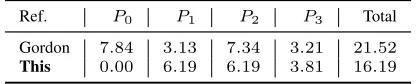
have to be online throughout the online phase, we can shut the server down for most of the online phase. Aided by this fact, the total monetary cost, which would be the total cost of hiring 4 servers to run our framework for either the training or prediction phase of an algorithm, we come out ahead of ABY3, primarily because the total running time of the servers in our framework is much lower. More details about monetary cost are presented in Appendix E.

Offline-online paradigm:To improve efficiency, a class of MPC protocols operates in the offline-online paradigm [28]. Data-independent computations are carried out in the offline phase, doing so paves way for a fast and efficient online phase of the protocol. Moreover, since the computations performed in the offline phase are data-independent, not all the parties need to be active throughout this phase, placing less reliance on each party. This paradigm has proved its ability to improve the efficiency of protocols in both theoretical [28]–[33] and practical [4], [34]–[41] domains. It is especially useful in a scenario like MLaaS, where the same functions need to be performed many times and the function descriptions are known beforehand. Furthermore, we operate in the outsourced setting of MPC, which allows for an arbitrary number of parties to come together and perform their joint computation via a set of servers. Each server can be thought of as a representative for a subset of data owners, or as an independent party. The advantage of this setting is that it allows the framework to easily scale for a large number of parties and the security notions reduce to that of a standard 4PC between the servers. Rings vs Fields: In the pursuit of practical efficiency, protocols in MPC that operate over rings are preferred to ones that work over finite fields. This is because of the way computations are carried out in standard 32/64-bit CPUs. Since these architectures have been around for a while, many algorithms are optimized for them. Moreover, operating over rings means that we do not have to override basic operations such as addition and multiplication, unlike with finite fields.

Although MPC techniques have been making a lot of progress towards being practically efficient, we cannot directly use the current best MPC protocols to perform PPML. This is mainly due to two reasons, which are:

1) MPC techniques operate in three different worlds – Arith-metic, Boolean, and Garbled. Each of these worlds is naturally better suited to carry out certain types of computations. For example, the Arithmetic domain (over a ring _Z2`) is more

suited to perform addition whereas the Garbled world is more suited to perform division. Activation functions used in machine learning, such as Rectified Linear Unit (ReLU), have operations that alternate between multiplications and comparisons. Operating in only one of the worlds, as most of the current MPC techniques do, does not give us the maximum possible efficiency. The mixed protocol framework for MPC was first shown to be practical by TASTY [42], which combined Garbled circuits and homomorphic encryption. The idea was later applied to the ML domain by SecureML [2], ABY3 [5] etc., where protocols to switch between the three worlds were proposed. These mixed world frameworks have proven to be orders of magnitude more efficient than operating in a single world.

(3)

machine learning are decimal numbers, we embed them over a ring by allocating the least significant bits to the fractional part. But several multiplications performed may lead to an overflow. A naive solution to avoid this is to use a large ring to accommodate a fixed number of multiplications, but the number of multiplications for machine learning varies based on the algorithm, making this infeasible. SecureML tackled this problem through truncation, which approximates the value by sacrificing the accuracy by an infinitesimal amount, performed after every multiplication. This technique, however, does not extend into the 3PC or 4PC setting, due to the attack described in ABY3, requiring us to come up with new techniques. Frameworks such as SecureML and ABY3 have tackled both these issues in the honest majority setting by proposing ways to switch between the three worlds efficiently, as well as efficient ways to do truncation. ABY3 is a lot more efficient than SecureML, in large part due to the 3PC primitives it uses. But ABY3 cannot avoid some expensive operations such as evaluation of a Ripple Carry Adder (RCA) in its truncation and activation functions. Truncation and activation functions – ReLU and Sigmoid, need rounds proportional to the underlying ring size in ABY3. This gives a lot of scope for improvement in the efficiency, which we achieve through our 4PC framework. A. Our Contribution

We propose an efficient framework for mixed world com-putations in the four-party honest majority setting with active security over the ring Z2`. Our protocols are optimized for

PPML and follow the offline-online paradigm. Our improve-ments come from having an additional honest party in the protocol. Our contributions can be summed up as follows: 1) Efficient 4PC Protocol: We propose an efficient four-party protocol with active security which proceeds through a masked evaluation inspired by Gordon et al. [26]. Our protocol requires

3 ring elements in the online phase per multiplication as opposed to 4 of [26], achieving a 25% improvement. This improvement is achieved by not compromising on the total cost (6 ring elements). Another significant advantage of our protocol is that the fourth party is not required for evaluation in the online phase. This is not the case with [26], where all the parties need to be online throughout the protocol exe-cution. In addition to the stated contributions, our framework also achieves fairness without affecting the complexity of a multiplication gate.

2) Fast Mixed World Computation: We propose a framework – Trident, that is geared towards a high throughput online phase as compared to the existing alternatives. This throughput is achieved by making use of an additional honest party. Every one of the conversions we propose to switch between the worlds is more efficient in terms of online communication complexity as compared to ABY3, with our improvements ranging from2×to2κ/3×, whereκdenotes the computational security parameter. More concretely, if we aim for 128-bit computational security, our framework gives a maximum im-provement of ≈85×. For instance, the technique we propose to perform bit composition (B2A) requires only 1 round, as opposed to1 + log`rounds in ABY3, which translates to a7×

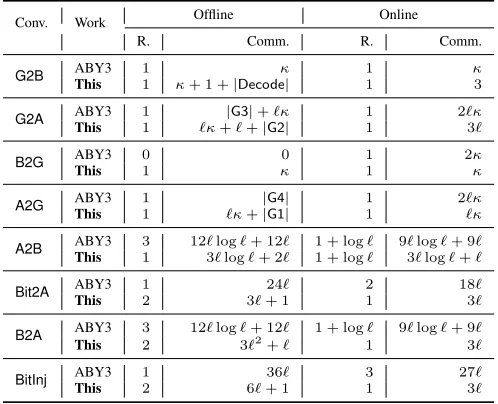
gain for a 64-bit ring. The table below provides the concrete cost of our online phase in comparison to ABY3. The overall cost comparison can be found in Table IX.

Conversion Ref. Rounds Communication

G2B ABY3 1 κ

This 1 3

G2A ABY3 1 2`κ

This 1 3`

B2G ABY3 1 2κ

This 1 κ

A2G ABY3 1 2`κ

This 1 `κ

A2B ABY3 1 + log` 9`log`+ 9` This 1 + log` 3`log`+`

B2A ABY3 1 + log` 9`log`+ 9`

This 1 3`

Table I: Online cost of share conversions of ABY3 [5] and This work.`denotes the size of underlying ring in bits andκdenotes the computational security parameter.

3) Efficient Truncation: The highlight of the protocol we propose for truncation is that it can be combined with our multiplication protocol with no additional cost in the online phase. In contrast, the online cost for multiplication in ABY3 increases from 9 to 12 ring elements, which gives us a 4×

improvement in online communication. Moreover, we forgo the need for (2` −2)-round Ripple Carry Adders (RCA), as opposed to ABY3, in the offline phase resulting in an improvement of 63×in rounds for a 64-bit ring.

Conversion Ref. Rounds Communication

Multiplication with Truncation

ABY3 1 12`

This 1 3`

Secure Comparison

ABY3 log` 18`log`

This 3 5`+ 2

Bit2A

JbK B_→

JbK

ABY3 2 18`

This 1 3`

BitInj

JbK B

JvK→JbvK

ABY3 3 27`

This 1 3`

ReLU ABY3_This 3 + log₄` ₈_`_{+ 2}45`

Sigmoid ABY3 4 + log` 81`+ 9

This 5 16`+ 7

Table II: Online cost of ML conversions of ABY3 [5] and This work.`denotes the size of underlying ring in bits.

4) Secure Comparison: We propose an efficient instantiation of secure comparison, with constant round complexity. ABY3 in comparison uses an optimized Parallel Prefix Adder (PPA), which takes log` rounds in the online phase. This amounts to2×improvement in the online rounds for a 64-bit ring. We also improve the online communication complexity by≈21×.

5) ML Building Blocks: The building blocks for ML high-lighted in the Table II (more details in Table X), have im-provements ranging from2×-3×in the round complexity and

(4)

6) Implementation: We implement all the stated protocols and test them over LAN and WAN. We benchmark the training and prediction phases of the algorithms – Linear Regression, Lo-gistic Regression, Neural Networks (NN), and Convolutional Neural networks (CNN). In order to compare with ABY3, we implement their protocols as well and obtain the benchmarks in our environment. For the training phase of Linear Regression, we have improvements across different configurations in the range of 2× to 251.84×. Similarly, for Logistic Regression, our improvements lie in the range of 2.71×to 67.88×. The respective range of improvements for NN and CNN are2.94×

-68.04× and3.19×-45.64×. Table IIIgives the concrete gain of the aforementioned algorithms over the most widely used MNIST dataset [43], which has 784 features, implemented with a batch size of 128. Moreover, our framework is able to process23online iterations of NN in a second for a batch size of 128, over LAN. This is a huge improvement over ABY3, which can process only 2.5 iterations, that too in the semi-honest setting. Similarly, for CNN, we could process 10.46

iterations as opposed to 2 of ABY3.

Network Linear

Regression

Logistic

Regression NN CNN

LAN 81.08× 27.07× 68.08× 45.64×

WAN 2.17× 2.76× 2.97× 3.19×

Table III: Gain in online throughput for ML Training over ABY3 [5] ford= 784features and batch size of 128.

We also provide results for the prediction phase and give throughput (no. of predictions per second) comparison details for the aforementioned algorithms, using real-world datasets. The gain in online throughput for prediction ranges from 3×

to 145.18× for Linear Regression and 3× to 158.40× for Logistic Regression over LAN and WAN combined. Similarly, the online throughput gain ranges from 335.44×to421.72×

for NN and 598.44×to759.65×for CNN.

II. PRELIMINARIES ANDDEFINITIONS

We consider a set of four parties P = {P0, P1, P2, P3}

that are connected by pair-wise private and authentic channels in a synchronous network. The function f to be evaluated is expressed as a circuit ckt, whose topology is publicly known and is evaluated over either an arithmetic ring Z2`

or a Boolean ring Z21, consisting of 2-input addition and

multiplication gates. The term D denotes the multiplicative depth of the circuit, while I,O,A,M denote the number of input wires, output wires, addition gates and multiplication gates respectively in ckt.

We use the notation wv to denote a wire w with valuev flowing through it. We use g = (wx,wy,wz,op) to denote a gate in the ckt with left input wirewx, right input wire wy, output wire wz and operationop, which is either addition (+) or multiplication (×).

For a vector~x,xidenotes theith_{element in the vector. For}

two vectors ~x and~y of lengthd, the dot product is given by, ~

x~y=Pd

i=1xiyi. Given two matrices X,Y, the operation X◦Ydenotes the matrix multiplication.

a) Shared Key Setup: In order to facilitate non-interactive communication, parties use functionality Fsetup that establishes pre-shared random keys for a pseudo-random function (PRF) among them. Similar setup for the three-party case can be found in [4], [5], [11], [12], [25].

In our protocols, we make use of acollision-resistanthash function, denoted byH(), to save communication. We defer the formal details of key setup and hash function to Appendix A.

III. OUR4PC PROTOCOL

In this section, we provide details for our 4PC protocol. We begin with the sharing semantics in Section III-A followed by explaining the relevant building blocks in Section III-B. We elaborate on the stages of our protocol in Section III-C. Lastly, in SectionIII-D, we show how to improve the security to achieve fairness.

A. Sharing Semantics

In this section, we explain three variants of secret sharing that are used in this work. The sharings work over both arithmetic (_Z2`) and boolean (_Z₂1) rings.

a)[·]-sharing: A valuevis said to be[·]-shared among parties P1, P2, P3, if the parties P1, P2 and P3 respectively hold the values v1,v2 andv3 such that v=v1+v2+v3. We use [·]_P

i to denote the [·]-share of party Pi for i∈ {1,2,3}.

b)h·i-sharing: A valuevis said to beh·i-shared among parties P1, P2, P3, if the parties P1, P2 and P3 respectively holds values(v2,v3),(v3,v1)and(v1,v2)such that v=v1+

v2+v3. We denoteh·i-shares of the parties as follows:

hviP1= (v2,v3), hviP2= (v3,v1), hviP3 = (v1,v2)

c)_J·_K-sharing: A valuevis said to be_J·_K-shared among parties P0, P1, P2, P3, if

– there exist valuesλv,mv∈Z2` such thatmv=v+λv. – parties P1, P2, P3 know the value mv in clear, while the

value λv ish·i-shared among them.

– partyP0 knowsλv,1, λv,2 andλv,3 in clear. We denote the J·K-shares of the parties as follows:

JvKP0= (λv,1, λv,2, λv,3) JvKP1 = (mv, λv,2, λv,3)

JvKP2= (mv, λv,3, λv,1) JvKP3 = (mv, λv,1, λv,2)

We useJvK= (mv,hλvi)to denote the J·K-share ofv.

d) Linearity of the secret sharing schemes: Given the

[·]-sharing ofx,yand public constantsc1, c2, parties can locally compute [c1x+c2y] =c1[x] +c2[y].

[c1x+c2y] = (c1x1+c2y1, c1x2+c2y2, c1x3+c2y3)

=c1[x] +c2[y]

It is easy to see that the linearity trivially extends to

h·i-sharing as well. That is hc1x +c2yi = c1hxi+c2hyi. Similarly, given the _J·_K-sharing of x,y and public constants c1, c2, parties can locally compute Jc1x+c2yK. Note that the

(5)

B. Building Blocks

a) Sharing Protocol: Protocol ΠSh (Fig. 1) enables party Pi to generate J·K-share of value v. The offline phase

is done using the pre-shared keys in such a way that Pi will

get the entire mask λ. During the online phase,Pi computes mv and sends to P1, P2, P3 who exchange the hash values to check for consistency.

Offline:

– IfPi=P0, parties inP \ {Pj}together sample λv,j forj∈ {1,2,3}.

– If Pi = Pk for k ∈ {1,2,3}, parties in P together sample

λv,k. In addition, parties inP \ {Pj} together sampleλv,j for

j∈ {1,2,3} \ {k}.

Online:

– Picomputesmv=v+λv and sends toP1, P2, P3.

– P1, P2, P3mutually exchangeH(mv)andabortif the received values are inconsistent.

ProtocolΠSh(Pi,v)

Figure 1:_J·_K-sharing of a valuevby partyPi.

Looking ahead, we also encounter scenarios where party P0 has to generate h·i-sharing of a value v in the offline phase. We call the resultant protocol as ΠaSh and the formal details appear in Fig.2.

Offline:

– Parties inP \ {P1}sample randomv1∈Z2`, while parties in

P \ {P2}sample randomv2.

– P0computesv3=−(v+v1+v2)and sends it to bothP1and

P2, who exchangeH(v3)andabortif there is a mismatch.

ProtocolΠaSh(P0,v)

Figure 2:h·i-sharing of a valuevby partyP0.

b) Reconstruction Protocol: Protocol ΠRec(P,v) (Fig.3) enables parties inP to computev, given its_J·_K-share. Towards this, each party receives the missing share from one other party and hash of the missing share from one of the other two parties. If the received shares are consistent, he/she will proceed with the reconstruction. Reconstruction towards a single party can be viewed as a special case of this protocol.

Online:

– P1 receivesλv,1 andH(λv,1)fromP2 andP0 respectively.

– P0 receivesmv andH(mv)fromP1 and P2 respectively.

Pifori∈ {0,1,2,3}abortif the received values are inconsistent. Else computesv=mv−λv,1−λv,2−λv,3.

ProtocolΠRec(P,_Jv_K)

Figure 3:Reconstruction of valuevamong parties inP.

C. Stages of our 4PC protocol

Our protocolΠ4PCconsists of three stages, namely – Input Sharing, Evaluation and Output Reconstruction. We elaborate on each of these stages below.

a) Input Sharing: For each wirewv holding the value

v, of whichPi∈ Pis the owner, he/she generatesJ·K-share of

v by executing theΠSh(Pi,v)protocol.

b) Evaluation: In this stage, parties evaluate the circuit in a topological order, where the following invariant is main-tained for every gate g: given the inputs of g in _J·_K-shared fashion, the output is generated in the J·K-shared fashion. For

the case of an addition gate g = (wx,wy,wz,+), the linearity of our sharing scheme maintains this invariant.

For a multiplication gateg= (wx,wy,wz,×), the protocol proceeds as follows: during the offline phase, partiesP1, P2, P3 locally compute[·]-shares ofγxy=λxλy, followed by exchang-ing them to form a h·i-sharing ofγxy. Before exchanging the shares of γxy, the parties randomize the shares by adding a share of0to the share ofγxyto prevent leakage. In addition,P0 helps the parties in verifying the correctness of shares received in the aforementioned step. During the online phase, the goal is to computemz. Note that,

mz=z+λz=xy+λz= (mx−λx)(my−λy) +λz

=mxmy−λxmy−λymx+λxλy+λz

Parties P1, P2, P3 locally compute [·]-share of mz −mxmy followed by an exchange to reconstruct mz−mxmy. By the nature of our secret-sharing scheme, every missing share can be computed by two parties. This facilitates the parties to verifiably reconstruct mz−mxmy by having one party send the missing share and the other send a hash of the same.

Each ofP1, P2, P3locally addmxmyto the result to obtain

mz. We call the resultant protocolΠMult (Fig.4).

Offline:

– Parties inP \ {Pj}together sampleλz,j forj∈ {1,2,3}. – Parties invoke protocolΠZero(Fig.22) to generateA, B,Γsuch

thatA+B+ Γ = 0. Parties locally compute the following: – P0, P1compute γxy,2=λx,2λy,2+λx,2λy,3+λx,3λy,2+A.

– P0, P2compute γxy,3=λx,3λy,3+λx,3λy,1+λx,1λy,3+B.

– P0, P3compute γxy,1=λx,1λy,1+λx,1λy,2+λx,2λy,1+ Γ.

– Parties exchange the following:

– P1 receivesγxy,3 andH(γxy,3)fromP2 andP0respectively.

– Pifori∈ {1,2,3}abortif received values are inconsistent.

Online:Letm0z=mz−mxmy.

– Parties locally compute the following:

– P1, P3compute m0z,2=−λx,2my−λy,2mx+γxy,2+λz,2.

– P1 receivesm0z,1 andH(m0z,1)fromP2 andP3 respectively.

– P2 receivesm0z,2 andH(m

0

(6)

0

z,3)fromP1 andP2 respectively.

– Pi for i ∈ {1,2,3} abort if the received values are

incon-sistent. Else, he / she computes mz= (m0z,1+m

0 z,2+m

0 z,3) + mxmy=m0z+mxmy.

Figure 4:Multiplication Protocol.

As a very important optimization, note that the exchange of hash values for every multiplication gate can be delayed until the output reconstruction stage. Moreover, all the corre-sponding values can be appended and hashed, resulting in an overall communication of only3 ring elements.

c) Output Reconstruction: For each of the output wire

wy with value y, parties execute protocol ΠRec(P,JyK) to

reconstruct the output.

Correctness and Security: We prove the correctness of

Π4PCbelow and defer the security details to Appendix F. Theorem III.1 (Correctness). ProtocolΠ4PC is correct.

Proof:We claim that for every wire inckt, the parties hold a_J·_K-sharing of the wire value inΠ4PC. The correctness for the input and output wires follows fromΠShandΠRecrespectively. The claim for addition gates follows from the linearity of_J·_K -sharing. For a multiplication gate g = (wx,wy,wz,×), when evaluated usingΠMult, the parties receivexy+λzin the online phase, resulting in obtainingJzK. The correctness ofxy+λzis

ensured through the verified reconstruction as shown inΠMult.

Theorem III.2 (Communication Efficiency). Π4PC requires one round with an amortized communication of 3M ring elements during the offline phase. In the online phase,Π4PC re-quires one round with an amortized communication of at most

3Iring elements in the Input-sharing stage,Drounds with an amortized communication of 3Mring elements for evaluation stage and one round with an amortized communication of3O

elements for the output-reconstruction stage.

D. Achieving Fairness

For fairness, we need to ensure that all the parties arealive in the protocol during the output reconstruction stage. On top of this, we also need to prevent the adversary from mounting a selective abort attack, where he can make some of the honest parties abort the protocol. To achieve this, parties P1, P2, P3 set a bitbtocontinue, if the verification of the multiplication gates was successful, else set it toabort, and send it toP0.P0 then sends abort back to all the parties if one of the parties sends abort, thus ensuring aliveness. Remaining parties then exchange their reply from P0 and follow the honest-majority in deciding whether to proceed or abort. Since there can be only 1 corruption, all the parties will now be on the same page, preventing a selective abort. If the parties decide to proceed, they exchange the missing shares. Using the fact that there is at most 1 corruption and the structure of our secret-sharing scheme, the most commonly received missing share will be consistent among the honest parties.

Online:

– P1, P2, P3 set bitb=abortif the verification for multiplica-tion fails. Else setb=continue.

– P1, P2, P3 sendbto P0 who sends backabort, if he/she re-ceives at least oneabortbit. Else sendscontinuetoP1, P2, P3. – P1, P2, P3 mutually exchange the message received fromP0. Partiesabortif the majority of the messages received areabort. Else they exchange the missing share as follows:

– P0 receivesmv fromP1, P2 andH(mv)fromP3 respectively. – P1 receivesλv,1 from P2, P3 and H(λv,1) from P0

respec-tively.

– P2 receivesλv,2 from P3, P1 and H(λv,2) from P0

respec-tively.

– P3 receivesλv,3 from P1, P2 and H(λv,3) from P0

respec-tively.

– Pifori∈ {0,1,2,3}chooses the missing share that forms the majority and computesv=mv−λv,1−λv,2−λv,3.

ProtocolΠfRec(P,JvK)

Figure 5:Fair reconstruction of valuevamong parties inP.

IV. MIXEDPROTOCOLFRAMEWORK

In this section, we present our mixed protocol framework, Trident. Before we go into the details of it, we discuss another world of MPC, called The Garbled World. To evaluate circuits over a ring Z2`, we operate in the arithmetic world and to

evaluate boolean circuits (_Z2`) we use either the boolean

world or the Garbled world, depending on the operation being performed. Superscripts {A, B, G} are used to indicate the respective worlds. If there is no superscript, the values are assumed to operate in the arithmetic world.

A. The Garbled World

For the Garbled world, we use the MRZ [16] scheme in the 4PC setting. In 4PC, parties P1, P2, P3 act as the garblers and the party P0 acts as the sole evaluator. As an optimisation, P0 can share his inputs with onlyP1, P2instead of all three parties. For cross-verification,P1sends the garbled circuit to P0 while P2 sends a hash of the it to P0. We incorporate the recent optimisations including free XOR [?], [44], [45], half-gates [46], [47], fixed-key AES garbling [48]. As opposed to the dishonest majority setting, this scheme removes the need for expensive public key primitives (in terms of communication) such as Oblivious Transfers altogether. We present the protocols for a single bit, and each operation can be performed` times in parallel to support`-bit values.

a) Sharing Semantics: For a bit v,JvK

G _{is defined as}

JvK

G

Pi =K

0

v ∈ {0,1}κfori∈ {1,2,3}andJvK

G

P0=K

v v=K0v⊕

vR, whereκis the computational security parameter. HereRis a globaloffsetwith the least significant bit as one, and is known only to P1, P2, P3 (generated by shared randomness), and R is common across all the _J·_KG_{-sharing. It is easy to see that} XOR of the least significant bit of _Jv_KG

P1 (resp.JvK

G

P2,JvK

G

P3)

and JvK

G

P0 is v. For a value v ∈ Z2`, we abuse the notation JvK

G_{to denote the set of}

J·K

(7)

Offline:

– P1, P2, P3 samples a randomK0

v ∈ {0,1}κ, computesK1v =

K0v⊕Rand setJvK G P1=JvK

G P2=JvK

G P3 =K

0

v. – P1, P2, P3 compute commitment of K0

v,K1v. P1, P2 send the commitments toP0 in a random permuted order, whoabortif the received commitments mismatch.

Online:

– PisendsK0v ⊕vRto P0, who sets it asJvK G P0.

– Pi decommits the right key Kvv to P0, who abort if the decommitment is incorrect.

ProtocolΠGSh(Pi,v)

Figure 6:_J·_KG_{-sharing of}_v_by _P

i fori∈ {1,2,3}.

b) Input Sharing: Protocol ΠG

Sh(Pi,v) enables Pi to

generate_J·_KG_{-sharing of value}_v_{. During the protocol,}_P 0needs to ensure that it obtains the correctKvv. To tackle this, we make the garblers commit both keys to P0, who can then verify the correctness by cross-checking the commitments received. The formal details for the case when Pi is one of the garblers

appear in Fig.6.

If Pi = P0, then ΠGSh(Pi,v) proceeds as follows: P0

samples random bit v1, computes v2 = v⊕v1 and sends v1 andv2 toP1 andP2 respectively. Parties executeΠGSh(P1,v1) and ΠG

Sh(P2,v2) to generate Jv1K

G _and

Jv2K

G _{respectively.} Parties then locally compute _Jv_KG ₌

Jv1K

G_⊕

Jv2K

G_{, using} the XOR gate evaluation method via the free-XOR technique. Here, the commitments of the keys need not be permuted, as P0already knows the actualv1andv2. As an optimization, the computation of _Jv1K

G_{can be offloaded to the offline phase.} c) Reconstruction: If Pi = P0, then P1, P2 send the least significant bit of their shares andPiverifies if it received

the same bit from bothP1andP2. IfPiis one of the garblers,

then P0 sends its share to Pi. Due to the authenticity of the

underlying garbling scheme [49], a corrupt P0 cannot send an incorrect share to Pi. If there are multiple reconstructions

towards Pi ∈ {P1, P2, P3}, P0 can send the least significant

bit of its shares along with a hash of all the corresponding shares.

d) Operations: Let u,v ∈ {0,1} be _J·_KG_{-shared with} P1, P2, P3 holding the shares (K0u,K0v), and P0 holding the shares (K0

u⊕uR,K0v⊕vR). Letcdenote the output. – XOR: The parties locally computeJcK

G₌

JuK

G_⊕

JvK

G_. – AND: P1, P2, P3 sample random K0

c ∈ {0,1}κ, compute

K1

u=K0u⊕Rand construct a garbled table for AND using the garbling scheme described in [46], [48].P1sends the garbled table to P0, while P2 sends a hash of the table to P0. P0 evaluates the table1 to obtain JcK

G

P0 =K

c

c.Pi fori∈ {1,2,3}

sets _Jc_KG_P

i =K

0 c. B. Building Blocks

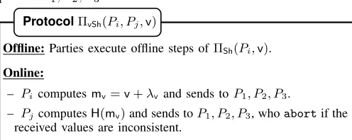
a) Verifiable Arithmetic/Boolean Sharing: Protocol

ΠvSh(Fig.7) allows two partiesPi, Pj to generateJ·K-sharing

of valuevin a verifiable manner. On a high level,Pi executes

1_{The garbled table can be send during the offline phase, while}_P 0needs to

evaluate the garbled circuit during the online phase.

ΠShonv, whilePj helps in verification by sendingH(mv)to parties P1, P2, P3.

Offline:Parties execute offline steps ofΠSh(Pi,v). Online:

– Picomputesmv=v+λv and sends toP1, P2, P3.

– PjcomputesH(mv)and sends toP1, P2, P3, whoabortif the received values are inconsistent.

ProtocolΠvSh(Pi, Pj,v)

Figure 7:Verifiable Arithmetic/Boolean sharing of a valuev.

We observe that the parties can non-interactivelygenerate

J·K-sharing of a valuevwhen all of the partiesP1, P2, P3know

v. Parties setλv,1=λv,2=λv,3= 0andmv=v. We abuse the notation and use ΠvSh(P1, P2, P3,v)to denote this protocol.

b) Verifiable Garbled Sharing: Protocol ΠG_vSh (Fig.8) is adapted from ABY3 [5] and allows two parties Pi, Pj to

generate_J·_KG_{-sharing of value}_v_{in a verifiable manner. When} Pi, Pj are both garblers, one of them can send the key while

the other can send just the hash to check for inconsistency. If P0=Pj, the other parties (P1, P2) send commitments of the keys in order, toP0. In addition,Pi sends the decommitment

of the actual key to P0.

Offline:P1, P2, P3 locally sample randomK0v ∈ {0,1} κ

, compute

K1

v =K0v⊕Rand setJvK G P1 =JvK

G P2=JvK

G P3=K

0

v.

Online:

– If(Pi, Pj) = (P1, P0):

– P1, P2 compute commitmentsCom(K0v),Com(K1v)and send it toP0. In addition,P1sends decommitment ofCom(Kvv)to

P0.

– P0 abortif either the received commitments are inconsistent

or the decommitment is incorrect. Else he/she sets_Jv_KG P0 =K

v v. – If(Pi, Pj) = (Pk, P0) fork ∈ {2,3}: The steps are similar

as above.

– If(Pi, Pj) = (P1, P2):P1andP2sendsKvvandH(K v v) respec-tively toP0, whoabortif the received values are inconsistent. Else he/she sets_Jv_KGP0=K

v v.

– If(Pi, Pj) = (P1, P3) or (P2, P3): The steps are similar as above.

ProtocolΠG

vSh(Pi, Pj,v)

Figure 8:Verifiable Garbled sharing of a valuev.

c) Dot Product: Given two vectors ~x and ~y, each of size d, ΠDotP (Fig. 9) computes the dot product z = ~x ~

(8)

Letz=~x~y.

Offline:

– Parties inP \ {Pj}together sampleλz,j forj∈ {1,2,3}. – Parties invoke protocolΠZero(Fig.22) to generateA, B,Γsuch

thatA+B+ Γ = 0. Parties locally compute the following: – P0, P1 computeγxy,2 =Pd_j₌₁γxjyj,2=

Pd

j=1(λxj,2λyj,2+ λxj,2λyj,3+λxj,3λyj,2) +A.

– P0, P2 computeγxy,3 =Pdj=1γxjyj,3= Pd

j=1(λxj,3λyj,3+ λxj,3λyj,1+λxj,1λyj,3) +B.

– P0, P3 computeγxy,1 =Pdj=1γxjyj,1= Pd

j=1(λxj,1λyj,1+ λxj,1λyj,2+λxj,2λyj,1) + Γ.

– P1 receivesγxy,3 andH(γxy,3)fromP2 andP0 respectively.

– Pifori∈ {1,2,3}abort if the received values are

inconsis-tent.

Online:Letm0z=mz−Pd_j₌₁mxjmyj.

– Parties locally compute the following: – P1, P3:m0z,2=

Pd

j=1(−λxj,2myj−λyj,2mxj) +γxy,2+λz,2.

– P2, P1:m0z,3= Pd

– P3, P2:m0z,1= Pd

– Parties exchange the following: – P1 receivesm0z,1 andH(m

0

– P2 receivesm0z,2 andH(m0z,2)fromP3 andP1 respectively.

0

– Pi for i ∈ {1,2,3} abort if the received values are

incon-sistent. Else, he / she computes mz= (m0z,1+m0z,2+m0z,3) + +Pd

j=1(mxjmyj) =m

0 z+

Pd

j=1(mxjmyj). ProtocolΠDotP(~x, ~y)

Figure 9:Dot Product Protocol.

C. Sharing Conversions

We now discuss the inter-sharing conversions among Arithmetic,Boolean, and Garbled sharing.

a) Garbled to Boolean Sharing (G2B): To convert a garbled share into the boolean world, P1, P2 first generate the garbled and boolean shares of a random value (r) using their shared randomness in the offline phase. In addition, they communicate the garbled circuit which performs the XOR of two bits along with the decoding information (Note that the garbled circuit does not have to be communicated due to the free XOR technique). In the online phase, P0 evaluates and obtains v⊕r and sends it to P3 along with the hash of the corresponding key. Authenticity of the underlying garbling scheme ensures that a corruptP0cannot send the wrong bit, as he will not be able to guess the right key for it.

Offline:

– P1, P2 locally sample random r ∈ Z2`. Parties execute ΠGvSh(P1, P2,r) and ΠBvSh(P1, P2,r) to generate JrK

G and JrK

B

respectively.

ProtocolΠG2B

– P1, P2, P3 garble a boolean adder circuitAdd(x,y) that com-putesx⊕y.P1sends the garbled circuit along with the decoding information toP0, whileP2 sends a combined hash toP0.

Online:

– P0 evaluates the circuitAdd on v and rto obtain v⊕r. P0

sendsv⊕ralong with a hash of the actual key corresponding

tov⊕rtoP3.P3abortif the received values are inconsistent.

– Else, parties executeΠBvSh(P3, P0,v⊕r)to generateJv⊕rK B

.

– Parties locally compute_Jv_KB=_Jv⊕r_KB⊕_Jr_KB.

Figure 10: Garbled to Boolean Sharing.

b) Garbled to Arithmetic Sharing (G2A): This conver-sion proceeds in a similar way asΠG2B. The major difference

is that instead of the garbled circuit for XOR, the parties communicate a circuit for subtraction of two`-bit values. Note thatP0needs to communicate only a single hash combining all the keys corresponding to the`-bits ofv−r.

Offline:

– P1, P2 locally sample random r ∈ Z2`. Parties execute ΠGvSh(P1, P2,r) and Π

A

vSh(P1, P2,r) to generate JrK G

and _Jr_KA

respectively.

– P1, P2, P3 garble a subtractor circuitSub(x,y) that computes

x−y. P1 sends the garbled circuit along with the decoding information toP0, whileP2 sends a combined hash toP0, who

abortif the received values are inconsistent.

Online:

– P0 evaluates the circuit Sub on v and r to obtain v−r. P0

sendsv−ralong with a combined hash of all the actual keys corresponding tov−r toP3. P3 abort if the received values are inconsistent.

– Else, parties executeΠA

vSh(P3, P0,v−r)to generateJv−rK A

.

– Parties locally compute_Jv_KA=_Jv−r_KA+_Jr_KA.

ProtocolΠG2A

Figure 11:Garbled to Arithmetic Sharing.

c) Boolean to Garbled Sharing (B2G): Since the bit

v= (mv⊕λv,1)⊕(λv,2⊕λv,3)in the boolean world, if we can get the garbled shares ofx= (mv⊕λv,1)andy= (λv,2⊕λv,3), parties can use the free XOR technique to compute the garbled shares of v locally. Each of x,y is possessed by two parties, enabling them to verifiably generate the garbled shares using the protocol ΠG

vSh.

Offline: P0, P1 execute ΠG

vSh(P1, P0,y) to generate JyK G

where

y=λv,2⊕λv,3.

Online:

– P2, P3 execute ΠG

vSh(P2, P3,x) to generate JxK

G _where _x ₌

mv⊕λv,1.

– Parties locally computeJvK G₌

JxK G_⊕

JyK G

.

ProtocolΠB2G

(9)

d) Arithmetic to Garbled Sharing (A2G): Similar to

ΠB2G, v = (mv−λv,1)−(λv,2+λv,3) and the parties can verifiably generate the garbled shares of x= (mv−λv,1)and

y= (λv,2+λv,3)using ΠGvSh. In the online phase, the parties evaluate a garbled subtractor circuit to obtain the shares of

v=x−y.

Offline:

– P0, P1 execute ΠGvSh(P1, P0,y) to generate JyK G

where y = λv,2+λv,3.

– P1, P2, P3 garble a subtractor circuitSub(x,y)that computes

x−y. P1 sends the garbled circuit to P0, while P2 sends a hash of the same to P0, whoabort if the received values are inconsistent.

Online:

– P2, P3 execute ΠGvSh(P2, P3,x) to generate JxK G

where x = mv−λv,1.

– Parties compute _Jv_KG = _Jx_KG−_Jy_KG by evaluating circuit

Sub.

ProtocolΠA2G

Figure 13:Arithmetic to Garbled Sharing.

e) Arithmetic to Boolean Sharing (A2B): This conver-sion proceeds similarly to Π_A2G, the only difference being parties now generate boolean shares of x= (mv−λv,1) and

y= (λv,2+λv,3)and evaluate a boolean subtractor circuit in-stead to compute boolean shares ofv=x−y.

Offline: P0, P1 execute ΠBvSh(P1, P0,y) to generate JyK B

where

y=λv,2+λv,3.

Online:

– P2, P3 execute ΠB

vSh(P2, P3,x) to generate JxK B

where x = mv−λv,1.

– Parties computeJvK B ₌

JxK B₋

JyK B

by evaluating an `-bit Boolean subtractor circuitSub.

ProtocolΠA2B

Figure 14:Arithmetic to Boolean Sharing.

f) Bit to Arithmetic Sharing (Bit2A): Let u and v

denote the bitsλbandmbrespectively over the ringZ2`. Then,

b=mb⊕λb=v+u−2vu

Party P0 generates h·i-shares of u in the offline phase. To ensure the correctness of the shares, parties P1, P2, P3 check whether the following equation holds – (λb⊕rb)0=u+r0b− 2ur0_b where the superscript(0) denotes the corresponding bits over ring Z2`. After the verification, parties locally convert hui to _Ju_K. In the online phase, parties multiply _Ju_K,_Jv_K to generate _Juv_K followed by locally computing _Jb_K = _Jv_K+ JuK−2JuvK. Note that since λv is set to 0 while executing ΠSh(P1, P2, P3,v) protocol,γuv-sharing is not needed during multiplication.

Offline: Let u and λu,i denote the bits λb and λb,i respectively over the ringZ2`. Herei∈ {1,2,3}.

– P0executesΠaSh(P0,u)(Fig.2) to generatehui. Let the shares behuiP1 = (u2,u3),huiP2= (u3,u1), andhuiP3= (u1,u2).

– P1, P2, P3 performs the following check:

– P1, P2 sample a random ring elementrand a random bit rb. Letr0bdenotes the bitrbover ringZ2`.

– P1 computesx1=λb,3⊕rb,y1= (u2+u3)(1−2r0b) +r 0 b+r and sends(x1,y1)toP3.

– P2 computesy2=u1(1−2rb0)−rand sendsH(y2)toP3. – P3 computesx=λb⊕rb =x1⊕λb,1⊕λb,2 and abortif

H(x0−y1)6=H(y2). Herex0denotes the bitxover ringZ2`.

– If the verification succeeds, P1, P2, P3 converts hui to _Ju_K

locally by settingmu= 0andhλui=−hui.

Online:Letvdenotes the bitmbover ringZ2`.

– Parties executeΠvSh(P1, P2, P3,v)to generateJvK. – Parties executeΠMultonJuKandJvKto generateJuvK.

– Parties locally compute_Jb_K=_Jv_K+_Ju_K−2_Juv_K.

ProtocolΠBit2A

Figure 15: Bit to Arithmetic Sharing.

g) Boolean to Arithmetic Sharing (B2A): We use the fact that a valuevcan be expressed as P`−1

i=02

i_·_vi_{, where} _vi

denotes the ith bit of vover a ring_Z2`. Note that

v= `−1

X

i=0

2i·vi = `−1

X

i=0

2i·(m0_v_i+λ0_u_i−2m0_v_i·λ0_u_i)

where m0_v_i and λ0_u_i denote the bits mvi and λui respectively

over the ring Z2`.

The offline phase ofΠB2Aproceeds similar toΠBit2A, where

each bit λvi for i ∈ {0, . . . , `−1} is converted to h·i-share.

During the online phase, parties locally compute [·]-shares of v followed by generating _J·_K-shares of it by executing

ΠvSh protocol. Parties then locally add their shares to obtain JvK.

Offline: Let vi denotes the ith bit of valuev. Let pi and λpi,j

denote the bitsλvi andλvi,j respectively over the ringZ2`, where i∈ {0, . . . , `−1}and j∈ {1,2,3}.

– Parties execute offline steps of ΠBit2A on each pi for i ∈ {0, . . . , `−1}, to generate hpii. Let the shares be hpiiP1 = (pi,2,pi,3),hpiiP2 = (pi,3,pi,1), andhpiiP3 = (pi,1,pi,2).

Online:Letqifori∈ {0, . . . , `−1}denotes bitmvioverZ2`.

– Parties compute the following: – P1, P3compute x=P`−1

i=02

i

(qi+pi,2−2qi·pi,2).

– P2, P1compute y=P`−1

i=02

i

(pi,3−2qi·pi,3).

– P3, P2compute z=P`−1

i=02

i

(pi,1−2qi·pi,1).

– Parties generate_Jx_K,_Jy_Kand_Jz_Kby executingΠvSh(P1, P3,x),

ΠvSh(P2, P1,y)andΠvSh(P3, P2,z)respectively. – Parties locally compute_Jv_K=_Jx_K+_Jy_K+_Jz_K.

ProtocolΠB2A

(10)

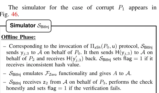
h) Bit Injection (BitInj): _Jb_KB

JvK → JbvK: Let y1 and

y2 denote the values λb andλbλv respectively over ringZ2`.

Similarly, letx0,x1,x2andx3denote the values(mbmv),(mb),

(mv−2mvmb)and(2mb−1)respectively over ringZ2`. Then,

b·v= (mb⊕λb)(mv−λv) =x0−x1y1+x2y2+x3y3

Offline:Lety1andy2 denote the valuesλbandλbλvrespectively overZ2`.

– P0 executesΠaSh(P0,yj) to generatehyjiforj∈ {1,2}. Let the shares be hyjiP1 = (yj,2,yj,3), hyjiP2 = (yj,3,yj,1), and

hyjiP3= (yj,1,yj,2).

– Parties verify the correctness ofhy1i using the steps similar to protocol ΠBit2A (Fig.15). To verify the correctness of hy2i, parties proceed as follows:

– Parties execute ΠZero (Fig.22) to generateA, B,Γsuch that

A+B+ Γ = 0.

– P1 computesu2=λy1,2λv,2+λy1,2λv,3+λy1,3λv,2+A.

– P2 computesu3=λy1,3λv,3+λy1,3λv,1+λy1,1λv,3+B.

– P3 computesu1=λy1,1λv,1+λy1,1λv,2+λy1,2λv,1+ Γ.

– P1 and P2 send z2 and H(−z3) respectively to P3, where

z2 =u2−y2,2 andz3=u3−y2,3.

– P3 setsz1=u1−y2,1 andabortifH(z1+z2)6=H(−z3).

Online: Let x0,x1,x2 and x3 denote the values (mbmv), (mb),

(mv−2mvmb)and (2mb−1)respectively over ringZ2`.

– Parties compute the following:

– P1, P3 computec2=x0−x1λv,2+x2y1,2+x3y2,2.

– P2, P1 computec3=−x1λv,3+x2y1,3+x3y2,3.

– P3, P2 computec1=−x1λv,1+x2y1,1+x3y2,1.

– Parties execute ΠvSh(P1, P3,c2), ΠvSh(P2, P1,c3) and

ΠvSh(P3, P2,c1)to generateJc2K,Jc3KandJc1Krespectively. – Parties locally compute_Jbv_K=_Jc1_K+_Jc2_K+_Jc3_K.

ProtocolΠBitInj

Figure 17: Bit Injection:_Jb_KB_Jv_KA→_Jbv_KA.

In the offline phase,P0generatesh·i-shares ofλ0bandλbλv whereλ0_bdenotes the bitλboverZ2`. The check forhλ0_biis the

same as the one forΠ_Bit2A, to checkhλbλviparties proceed as mentioned in protocol ΠBitInj above. During the online phase,

parties locally compute[·]-shares ofb·vfollowed by generating

J·K-shares of it by executingΠvShprotocol. Parties then locally

add their shares to obtain _Jb·v_K.

V. PRIVACYPRESERVINGMACHINELEARNING Most of the intermediate values in machine learning algo-rithms involve operating over decimals. To represent decimal values, we use signed two’s compliment overZ2` [2], [5], [25],

where the most significant bit (msb) represents the sign and the last dbits represent the fractional part.

In order to perform privacy-preserving machine learning, we need efficient instantiations of three components – Share Truncation, Secure Comparison, and Non-linear Activation Functions. This section covers our protocols for performing the aforementioned components.

A. Share Truncation

We take inspiration for truncation from ABY3 [5], where they perform it on shares after evaluating a multiplication gate, preserving the underlying value with very high probability. Our approach improves upon ABY3 by not using any boolean cir-cuits, thus improving the offline round complexity to constant.

Offline:

– Parties execute the offline steps of protocolΠMult(wx,wy,wz) apart fromλznot being generated.

– Parties locally sample the following random values:

P \ {P2}:r2, P \ {P1}:r1, P \ {P3}:r3

– P0locally computer=r1+r2+r3, locally truncates it to obtain

rt and executes ΠaSh(P0,rt) to generatehrti. Let the shares be hrtiP1= (r

t

2,rt3),hrtiP2= (r

t

3,rt1), and hrtiP3 = (r

t

1,rt2).

– Letrd and rd,i denote the last dbits of r and ri respectively for i ∈ {1,2,3}. Parties verify the correctness of hrt_i

as follows:

– P1 samples a random elementc and computes m1 = r2−

2d_rt

2−rd,2+c.P1 sends(m1,H(c))toP2.

– P2 computesm2= (r1+r3)−2d(rt1+r

t

3)−(rd,1+rd,3)and

abortifH(m1+m2)6=H(c).

– Parties locally convert hrti to _Jrt_K by setting mrt = 0 and hλrti=hrti.

Online:Letz0= (z−r)−mxmy.

– Parties locally compute the following:

– P1, P3compute [z0]₂=−λx,2my−λy,2mx+γxy,2−r2.

– P2, P1compute [z0]₃=−λx,3my−λy,3mx+γxy,3−r3.

– P3, P2compute [z0]₁=−λx,1my−λy,1mx+γxy,1−r1.

– P1 receives[z0]₁ andH([z0]₁)fromP2 andP3 respectively. – P2 receives[z0]₂ andH([z0]₂)fromP3 andP1 respectively. – P3 receives[z0]₃ andH([z0]₃)fromP1 andP2 respectively.

– Pifori∈ {1,2,3}abortif the received values are

inconsis-tent. Else, he computes(z−r) = [z0]₁+ [z0]₂+ [z0]₃+mxmy.

– P1, P2, P3 locally truncates(z−r)to obtain(z−r)t

, followed by executingΠvSh(P1, P2, P3,(z−r)t)to generateJ(z−r)

t K. – Parties locally computeJz

t

K=J(z−r) t

K+Jr t

K.

ProtocolΠMultTr(wx,wy,wz)

Figure 18: Multiplication with Truncation.

We start by generating a random (r,rt₎ _{in the offline phase,} wherert is the truncated value ofr. The truncated value ofz

can be obtained by first opening and truncatingz−r, and then adding it tort_{. Parties non-interactively generate}_h_r_i_{, such that} P0obtainsr. This is followed byP0generating_Jrt

K, but since

we cannot rely on P0, partiesP1, P2, P3 perform a check to ensure the correctness of the share. On a high level, parties check the relation r= 2d_rt₊_r

d, where rd denotes the last d bits of r The formal details of the check are provided in the protocol above and the correctness appears in LemmaD.1. B. Secure Comparison

(11)

arithmetic, a simple way to achieve this is by computingx−y, and checking its sign, stored in themsbposition. This protocol, inspired from ASTRA [25], is called Bit Extraction (ΠBitExt), since it extracts a bit from the given arithmetic shares and outputs the boolean shares of the bit.

Offline:

– P1, P2 sample randomr∈Z2` and setx=msb(r).

– Parties executeΠvSh(P1, P2,r)andΠBvSh(P1, P2,x)to generate JrKandJxK

B

respectively.

Online:

– Parties executeΠMultonJrKandJvKto generateJrvK, followed by reconstructingrvtowardsP0 and P3.

– P3, P0sety=msb(rv)followed by executingΠBvSh(P3, P0,y) to generate_Jy_KB.

– Parties locally compute_Jmsb(v)_KB₌ JxK

B_⊕ JyK

B_.

ProtocolΠBitExt(P,JvK)

Figure 19: Extraction of MSB bit of valuev.

C. Activation Functions

a) ReLU: The ReLU function is defined as relu(v) = max(0,v). This can be viewed asrelu(v) = (1⊕b)vwhere bit

b= 1ifv<0and0otherwise. In order to generate_Jrelu(v)_K, parties first execute ΠBitExt on v to obtain JbK

B _{and locally} compute _J1⊕b_KB_{. This is followed by executing} _Π

BitInj on J1⊕bK

B_and

JvK. The derivative ofrelu, denoted bydrelu(v) = (1⊕b).

b) Sigmoid: In our protocols, we use the approximation of sigmoid function [2], [5], [25], defined as:

sig(v) =

  

0 v<−1

2

v+1₂ −1 2 ≤v≤

1 2

1 v>1₂

This can be viewed as,sig(v) = (1⊕b1)b2(v+1/2)+(1⊕b2), whereb1= 1ifv+ 1/2<0andb2= 1if v−1/2<0. The protocol is similar to that of relu apart from an additional bit extraction, bit multiplication and a bit injection is required.

VI. IMPLEMENTATION ANDBENCHMARKING The improvements of our framework over the current state-of-the-art (ABY3) are showcased through our implementa-tion, comparing the two. The training and prediction phases of Linear Regression, Logistic Regression, Neural Networks (NN), and Convolutional Neural Networks (CNN) are used for benchmarking. While we compare our construction with the malicious ABY3 in this section, the comparison of ours with the semi-honest version of ABY3 and with the 4PC protocol of Gordon et al. [26] are deferred to AppendixE.

a) Environment Details: We provide results for both LAN (1Gbps bandwidth) and WAN (40Mbps bandwidth) set-tings. In the LAN setting, we have machines with 3.6 GHz Intel Core i7-7700 CPU and 32 GB RAM. In the WAN setting, we use Google Cloud Platform2with machines located

2_{https://cloud.google.com/}

in West Europe (P0), East Australia (P1), South Asia (P2) and South East Asia (P3). We use n1-standard-8 instances, where machines are equipped with 2.3 GHz Intel Xeon E5 v3 (Haswell) processors supporting hyper-threading, with 8 vCPUs, and 30 GB RAM. We measured the average round-trip time (rtt) for communicating 1 KB of data between every pair of parties. Over the LAN setting, the rttturned out to be

0.296ms. In the WAN setting, therttvalues were

P0-P1 P0-P2 P0-P3 P1-P2 P1-P3 P2-P3

274.83ms 174.13ms 219.45ms 152.3ms 60.19ms 92.63ms

We implement our protocols using the ENCRYPTO li-brary [50] in C++17 over a 64 bit ring. Since the codes for ABY3 and MRZ [16] are not publicly available, we implement their protocols in our environment. The hash function is instantiated using SHA-256. We use multi-threading, wherever possible, to facilitate efficient computation and communication among the parties. To even out the results, each experiment is run 20 times and the average values are reported.

b) Datasets: To benchmark the training phase of ma-chine learning algorithms, it is common practice to use synthetic datasets so that we have freedom to choose the parameters of the datasets. However, testing the accuracy of a trained model must be carried out with a real dataset, which is the MNIST [43] in our case. It contains28×28pixel images of handwritten numbers and 784 features. For benchmarking of the prediction phase, we use the following real-world datasets: Dataset #features #samples

Candy (CD)Power Ranking [51] 13 85

Boston (BT)Housing Prices [52] 14 506

Weather (WR)Conditions in World War Two [53] 31 ≈119000 CalCOFI (CI)- Oceanographic Data [54] 74 ≈876000 Epileptic (EP)Seizures [55] 179 ≈11500

FoodRecipes (RE)[56] 680 ≈20000

MNIST [43] 784 70000

We choose Boston, Weather and CalCOFI for linear regression, since they are best suited for it, while Candy, Epileptic and Recipes were chosen for logistic regression. For NN and CNN, we used the MNIST dataset.

A. Secure Training

The training phase in most of the machine learning algo-rithms consists of two stages– i) forward propagation, where the model computes the output, and ii) backward propagation, where the model parameters are adjusted according to the computed output and the actual output. We define oneiteration in the training phase as one forward propagation followed by a backward propagation.

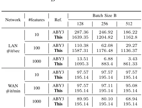
This section covers the improvements in the training phase of our protocol as compared to ABY3. We report the per-formance in terms of the number of iterations over varying feature (d) and batch sizes (B), whered∈ {10,100,1000}and B ∈ {128,256,512}. In LAN, we use iterations per second (#it/sec) as the metric, but sincerttis much higher for WAN, we instead use iterations per minute(#it/min).

(12)

Gradient Descent algorithm (GD). The update function for w~ is given by

~

w=w~ − α

BX

T

i ◦(Xi◦w~ −Yi)

where α denotes the learning rate and Xi denotes a subset

of batch size B, randomly selected from the entire dataset in the ith iteration. Here the forward propagation consists of computing Xi◦w~, while the weight vector is updated in the

backward propagation. The update function consists of a series of matrix multiplications, which in turn can be achieved using dot product protocols. The operations of subtraction as well as multiplication by a public constant can be performed locally. We observe that the aforementioned update function can be computed entirely in the arithmetic domain and can be viewed in form ofJ·K-shares as

Jw~K=Jw~K−

α BJX

T

jK◦(JXjK◦Jw~K−JYjK)

Network #features Ref.

Batch Size B

128 256 512

LAN #it/sec

10 ABY3 287.36 246.92 186.22 This 1639.35 1204.82 1162.8

100 ABY3 110.38 62.08 29.27 This 1587.31 1176.48 1136.37

1000 ABY3 13.51 6.88 3.43 This 1095.3 883.4 861.33

WAN #it/min

10 ABY3 97.57 97.57 97.57 This 195.14 195.14 195.14

100 ABY3 97.57 97.11 95.08 This 195.14 195.14 195.14

1000 ABY3 89.95 80.10 68.94 This 195.14 195.14 195.14

Table IV: Comparison of ABY3 (Malicious) and This for Linear Regression (higher = better).

Table IV provides concrete values for Linear Regression. Our improvement over LAN ranges from 4.88× to251.84×

and 2× to 2.83× over WAN. The gain comes due to two factors: One being the amount we save through our feature-independent communication of the dot product protocol (3ring elements as opposed to 9d). The other factor is our efficient truncation protocol, which reduces the online communication from12elements to3 elements – by75%. The reason for the discrepancy in gains in LAN and WAN is because in LAN, the rtt is in the order of microseconds, and scales with the communication size. In contrast, therttin WAN is in the order of milliseconds and does not scale with communication up to a threshold, within which all our protocols operate.

b)Logistic Regression: The iteration for the case of logistic regression is similar to that of linear regression, apart from an activation function being applied on Xi◦w~ in the

forward propagation. We instantiate the activation function using sigmoid (Section V-C). The update function for w~ is given by

~

w=w~ − α

BX

T

i ◦(sig(Xi◦w)~ −Yi)

One iteration of logistic regression incurs an additional cost for computing sig(Xj◦w)~ as compared with that for linear

regression.

Network #features Ref. Batch Size B

128 256 512

LAN #it/sec

10 ABY3_This _338.9956.95 _257.0142.02 _226.6130.35

100 ABY3 43.34 27.89 16.2 This 336.71 255.69 225.64

1000 ABY3 11.36 6.06 3.13 This 307.41 238.44 212.23

WAN #it/min

10 ABY3 20.54 20.54 20.52 This 55.76 55.76 55.76

100 ABY3 20.54 20.52 20.41 This 55.76 55.76 55.76

1000 ABY3_This 20.18_55.76 19.64_55.76 18.87_55.76

Table V: Comparison of ABY3 (Malicious) andThis for Logistic Regression (higher = better).

TableVprovides concrete values for Logistic Regression. Logistic Regression can be thought of as an execution of Linear Regression followed by a Sigmoid function on the output, due to which our improvements for Linear Regression carry over to Logistic. Our improvement ranges from 5.95×

to 67.88× over LAN and 2.71× to 2.96× over WAN. Our efficient Sigmoid protocol takes this result further by improv-ing upon the round and communication complexity. The round complexity is brought down to constant from 4 + log` to5. Instantiated over ringZ264, this amounts to an improvement of 50%. The communication is also improved by ≈80% (from

81 elements to roughly16).

c)Neural Networks: For the case of NN, we follow steps similar to that of ABY3, where each node across all the layers, except the last layer, uses ReLU (relu) as the activation function. At the output layer, we use the MPC friendly vari-ant of the softmax activation function, smx(ui) = Pnfrelu(ui)

j=1relu(uj) , proposed by SecureML [2]. In order to perform the division, we switch from arithmetic to garbled world and then use a division garbled circuit.

The network is trained using the Gradient Descent, where the forward propagation comprises of computing activation matrices for all the layers in the network. Here, the activation matrix for all the layers except the output, is defined as

Ai =relu(Ui), whereUi=Ai−1◦Wi .A0is initialized to

Xj, whereXj is a subset of batch sizeB, randomly selected

from the entire dataset for the jth _{iteration. The activation}

matrix for the output layer is defined as Am=smx(Um). During the backward propagation, error matrices are com-puted first. The error matrix for the output layer is defined as Em = (Am−T), while for the remaining layers it is

defined asEi= (Ei+1◦WiT)⊗drelu(Ui). Here the operation

⊗ denotes element wise multiplication anddrelu denotes the derivative of ReLU. This is followed by updating the weights as Wi=Wi−_BαATi−1◦Ei.

(13)

Network Ref.

LAN (#it/sec) WAN (#it/min)

B-128 B-256 B-512 B-128 B-256 B-512

NN ABY3 0.37 0.25 0.15 4.69 4.28 3.87

This 23.00 13.55 7.70 13.94 13.94 13.79

CNN ABY3 0.23 0.18 0.13 4.34 4.05 3.71

This 10.46 5.63 2.99 13.86 13.67 13.16

Table VI: Comparison of ABY3 (Malicious) and Thisfor NN and CNN (higher = better).

involves one forward pass followed by one back-propagation. In LAN, the number of iterations is maximum with a batch of 128, at 22.99 #it/sec, and comes down to 7.70 with a batch size of 512. Similarly, over WAN it is maximum at 13.94

and comes down to 13.79. As expected, the #it/sec has not decreased with increase in features due to our dot product protocol being feature-independent in terms of communication. ABY3 on the other hand, has reported 2.5 #it/sec with a batch size of 128, in the computationally lighter semi-honest setting. Table VIabove provides more details.

We also considered a CNN discussed in [4] with 2 hidden layers, consisting of 100 and 10 nodes. Similar to ABY3, we overestimate the running time by replacing the convolutional kernel with a fully connected layer. In LAN, the number of iterations is maximum with a batch of 128, at 10.46 #it/sec, and comes down to 2.99with a batch size of 512. Similarly, over WAN it is maximum at13.86and comes down to13.16. B. Secure Prediction

For Secure Prediction, we use online latency of the protocol as a metric to compare both works. The units are milliseconds in LAN and seconds in WAN. We use the MNIST dataset, which has 784 features, with a batch size of 1 and 100 for benchmarking. Our truncation protocol causes a bit-error at the least significant bit position, which is the same as that of ABY3 and SecureML [2] due to similarity in the techniques. We refer the readers to SecureML for a detailed analysis of the bit-error. The accuracy of the prediction itself however, ranges from 93%for linear regression to 98.3%for CNN.

Network Batch Size Ref.

Linear Regression

Logistic

Regression NN CNN

LAN (ms)

1 ABY3 2.08 6.25 73.09 371.1

This 0.25 1.75 4.51 5.4 100 ABY3 37.80 49.68 1284.95 2010.06

This 0.30 2.55 17.17 39.63

WAN (s)

1 ABY3 0.47 2.77 6.02 6.25

This 0.16 0.93 2.31 2.31 100 ABY3 0.49 2.79 7.04 7.5

This 0.16 0.93 2.31 2.32

Table VII: Online Runtime of ABY3 (Malicious) and This for Secure Prediction of Linear, Logistic, NN, and CNN models for

d= 784. (lower = better).

For Linear Regression, our improvement ranges from 3×

to 126×, considering LAN and WAN together. For Logistic Regression, our improvement ranges from 3× to 19.48×, considering LAN and WAN together. In NN, we achieve an improvement ranging from 3.05× to 74.85×. Similarly for CNN, the improvement ranges from2.71×to68.82×.

Though not stated explicitly, our offline cost for linear regression is orders of magnitude more efficient as compared to ABY3. This improvement carries over for logistic regres-sion, NN, and CNN networks as well. A large part of this improvement comes from the difference in the approaches to truncation. ABY3’s approach entails using Ripple Carry Adder (RCA) circuits, which consume 128 rounds. ABY3 has pointed out that this was the reason SecureML performed better in total time for a single prediction. Our approach on the other hand, does not use any such circuit, resulting in an improvement of

≈15×in communication and64×in rounds.

Throughput Comparison: We use a different metric to better illustrate the impact of our efficiency in the case of secure prediction, which is online throughput. Online through-put over LAN is the number of predictions that can be made in a second, and over WAN it is the number of predictions per minute. We have a total of 32threads over4 CPU cores, wherein each thread can perform 100 queries simultaneously without reduction in performance. Table VIII provides the online throughput comparison of ABY3 and ours for secure prediction over real-world datasets in a LAN setting. The gains for linear regression range from26.16×to145.18×and from 5.69×to158.40×for logistic regression. Similarly, we observed gains of 335.44× and 598.44× for NN and CNN respectively.

Ref. Linear Regression Logistic Regression NN CNN BT WR CI CD EP RE MNIST

ABY3 4.08 1.74 0.73 2.20 0.29 0.08 0.46 0.06 This 106.67 106.67 106.67 12.55 12.55 12.55 153.39 37.43

Table VIII: Online Throughput Comparison of ABY3 (Malicious) and Thisfor Secure Prediction over LAN. (higher = better)

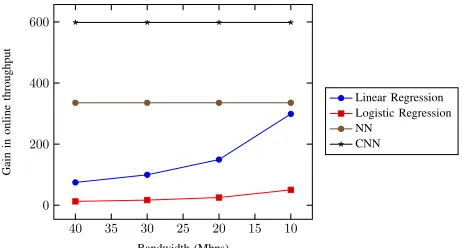
In WAN, even though our protocols are more communi-cation efficient as compared to ABY3, we could not fully capitalize on it especially for Linear Regression and Logistic Regression. This is due to the limitation of being able to run only 32 CPU threads in parallel, which amounts to a lot of bandwidth not being utilized. This gap can be closed by introducing more CPU threads into our infrastructure. However, since we could not do this, in order to showcase the efficiency better, we limit the bandwidth and compute the gain in online throughput. As evident from the plot in Fig.20, the gain increases as we limit the bandwidth. We observe that our protocols for Linear Regression and Logistic Regression achieve maximum bandwidth utilization at around 1.5 Mbps. On the other hand, NN and CNN utilize the entire bandwidth, even at 40 Mbps. So decreasing the bandwidth does have an effect on the throughput for NN and CNN.

VII. CONCLUSION