Confidence Interval Estimation for Precipitation Quantiles Based on Principle of Maximum Entropy

Confidence interval estimation for precipitation quantiles based

on principle of maximum entropy

Ting Wei Songbai Song*

College of Water Resources and Architectural Engineering, Northwest A&F University, Yangling, 712100, China.

* Correspondence: [email protected] (S.S.).

Abstract: Confidence interval of is an interval corresponding to a specified confidence and

including the true value. It can be used to describe the precision of a statistical quantity and

quantify its uncertainty. Although the principle of maximum entropy (POME) has been used

for a variety of applications in hydrology, the confidence intervals of the POME quantile

estimators have not been available. In this study, the calculation formulas of asymptotic

variances and confidence intervals of quantiles based on POME for Gamma, Pearson type 3

(P3) and Extreme value type 1 (EV1) distributions were derived. Monte Carlo Simulation

experiments were performed to evaluate the performance of derived formulas for finite samples.

Using four data sets for annual precipitation at the Weihe River basin in China, the derived

formulas were applied for calculating the variances and confidence intervals of precipitation

quantiles for different return periods and the results were compared with those of the methods

of moments (MOM) and of maximum likelihood (ML) method.It is shown that POME yields

the smallest standard errors and the narrowest confidence intervals of quantile estimators

among the three methods, and can reduce the uncertainty of quantile estimators.

Keywords: Principle of maximum entropy; quantile estimation; confidence interval; Monte

Carlo simulation; precipitation frequency analysis

1

Introduction

One of the objectives of hydrological frequency analysis is to estimate the magnitude of a

hydrologic event with a given return period [1,2]. The short record length of sample data and

the application of inappropriate distribution inevitably involve some uncertainties in this

estimation [3]. Hence, a point estimate of quantile corresponding to a return period is usually

not enough because it cannot adequately express the precision of the estimation. Confidence

interval can be used to describe the precision of a statistical quantity and it provides more

information than a point estimate. The calculation of confidence interval requires the results of

standard errors. Different estimation methods may yield different standard errors of the

estimated quantities, and thus the confidence intervals are different as well. The most efficient

method is the one that gives the smallest error and the narrowest confidence interval width [1].

Therefore, it is necessary to compare the performance of different methods and to choose the

most efficient method for improving the calculation accuracy of hydrological quantile

estimators.

There have been a multitude of studies related to the estimation of variances and

confidence intervals of estimated quantile estimators. Nash and Amorocho obtained the

expressions for the standard errors of flood quantile estimators for a given return period from

random samples of normal and double exponential population [4]. Bobee derived the formulas

of sampling error of T-year flood quantile computed by fitting a log-Pearson type-3 distribution

[5]. Assuming the design events are normally distributed, Kite derived the confidence limits of

design events using data generation experiments [6]. Condie gave the maximum likelihood

for asymptotic standard error of a T-year event and he concluded that the maximum likelihood

method is markedly superior to method of moments in the estimation of asymptotic standard

error of T-year event [7]. Lawless reviewed the methods for calculating the confidence interval

for parameters or other characteristics of the Weibull and extreme value distributions, and

compared performances of the various methods [8]. Hoshi and Barges developed an

approximation technique to compute the derivative of a standard gamma quantile with respect

to the distribution shape parameter for estimating the sampling variance of a specified quantile

[9]. They also derived the expressions for calculating the sampling variances and covariances

of log-Pearson type 3 distribution parameters as well as the sampling variance of T-year flood

event using the method of moments [10]. Phien derived the explicit formulas for the variances

and covariances of the parameter estimates of log-Pearson type 3 distribution when the method

of direct and mixed moments was used for parameter estimation [11]. Stedinger (1983), Ashkar

and Bobee (1988) also investigated several methods for calculating the confidence intervals for

P3 and log-Pearson type 3 quantiles and tested their performance [12,13]. Lu and Stedinger

derived the simple formulas for estimating the asymptotic variance of probability weighted

moments (PWM) quantile estimators for generalized extreme value (GEV) distribution when

the location and scale parameters were estimated with a fixed regional shape parameter or all

three parameters are estimated. They compared the variances of quantile estimators for the two

cases and examined the performance of the approximate confidence intervals obtained using

the derived formulas [14]. Sampling variance of normalized GEV/PWM quantile estimators

were also investigated by Lu and Stedinger [15]. Heo and Salas derived the confidence limits

from the method of moments (MOM), PWM method and maximum likelihood (ML) method,

and compared the applicability of the three estimation methods by using observed flood data.

They concluded that the MOM yielded narrower confidence limits than did the ML and PWM

methods especially for high return periods [16]. Ashkar presented an approximate procedure

for calculating confidence intervals of quantiles for gamma and generalized gamma

distributions, and tested its suitability by numerical applications. They found that the

approximate method performs well for hydrological applications where the data record is short

[17]. Heo et al. derived and compared the asymptotic variances and confidence intervals of

quantiles for the two- and three-parameter weibull distributions based on the MOM, ML, and

PWM methods [18]. Su investigated two parametric methods for computing the confidence

intervals of quantiles for generalized lambda distribution [19]. Shin summarized the parameter

estimation procedure for the generalized logistic distribution based on the MOM, ML, and

PWM, and derived the asymptotic variances of the MOM, ML, and PWM quantile estimators

for the generalized logistic distribution [20]. The confidence intervals of quantiles for

two-parameter Kappa distribution and heavy-tailed generalized Pareto distributions have also been

investigated[21,22].

Shannon defined the concept of entropy as a measure of uncertainty of a random variable

or its probability distribution [23]. Jaynes later formulated the principle of maximum entropy

(POME) which provides a rational approach to choose the most unbiased probability

distribution for hydrologic frequency analysis [24]. POME also provides a way to estimate

parameters of a given distribution from the specified constraints. The Shannon entropy and

probability distribution appropriate for hydrologic frequency analysis in the absence of a large

amount of data [25]. Singh developed a procedure for derivation of a number of frequency

distributions used in hydrology using POME, including the two- and three-parameter lognormal

distributions, extreme value type I and III distributions, generalized extreme value distribution,

Weibull distribution, P3 distribution, log-Pearson type 3 distribution, beta distribution, two- and

three-parameter log-logistic distributions, two- and three-parameter generalized Pareto

distributions and two-component extreme value distribution, etc [26]. He also summarized the

entropy method for parameter estimation for these distributions and indicated that the entropy

method is reasonable and efficient for parameter estimation [27]. Fiorentino derived a

parameter estimation method for the two component extreme value distribution based on the

POME and indicated that the POME method is suitable for both site-specific and regional

estimation [28]. Singh and Song applied POME to estimate parameters of the four-parameter

kappa distribution and the four-parameter exponential gamma distribution. The results of the

estimation show that the POME enables these two distributions to fit the data better than the

other estimation methods [29,30]. Chen derived the generalized distribution for flood and

extreme rainfall frequency analysis and she concluded that the entropy-based generalized

distributions are superior or comparable to other traditional distributions [31,32]. Hao

constructed the bivariate joint distribution of drought duration and severity using bivariate

entropy and results show that the entropy-based joint distribution is capable for bivariate

drought analysis. In recent years, an integration of entropy and copula has been developed to

construct the joint distribution function [33]. Hao proposed maximum entropy copula for

maximum entropy copula is very close to the observed streamflow [34]. Kong integrated POME

with Gumbel-Hougaard copula for monthly streamflow simulation. The simulation shows that

the variability of simulated monthly streamflow is similar to that of observed monthly

streamflow [35]. AghaKouchak reviewed the currently available maximum entropy copula

models and discussed their potential applications in hydrology and climatology. He applied the

entropy copula to bivariate flood frequency analysis to illustrate the construction of the bivariate

joint distribution using the entropy copula [36].

In variances estimation, Phien provided the formulas for calculating the approximate

variances and covariances of the parameter estimators and the approximate variance of the T

-year event obtained by POME for the extreme value type-1 (EV1) distribution. Through

applications of the formulas to simulated data, he concluded that the approximations for the

variance of estimates of the T-year event are of sufficient accuracy [37]. The sampling

properties of the maximum entropy estimators for P3 distribution has been investigated as well

[38]. The investigation concluded that the efficiency of the POME can be improved by using

biased estimator of the variance of variable. Despite the advances mentioned above, the POME

based confidence intervals of quantile estimators have not been investigated and the

performance of POME, MOM and ML in the estimation has not been compared.

The objective of this study is therefore to derive the formulas for calculating the confidence

intervals of quantiles based on POME for Gamma, P3 and EV1 distributions; evaluate the

performance of derived confidence intervals for finite samples using simulation experiments;

compute the confidence of annual precipitation quantiles for different return periods; and

2

Confidence interval estimation of the quantile

The standard error and confidence interval are two measures to describe the uncertainty of

a statistical quantity, such as the T-year quantile estimator

x

ˆ

_T. The standard error s_T measures

the standard deviation of an estimated quantile from a sample about the true value, and the

confidence interval of a quantile estimated by a sample is an interval that corresponds to a

specified confidence and includes the true value.

2.1 Estimation of quantile

A general form for calculating

x

ˆ

_T of a given distribution can be written in terms of the

distribution moments and the frequency factor K_T[39]:

2

1 ˆ

ˆ

ˆT



KT



x = + (1) where



ˆ

₁



and



ˆ

₂ are the mean and the standard error of the population, respectively, and they will equal to the sample moments only when the MOM is used for parameter estimation;

T

K is the frequency factor specific to the chosen distribution, which can be derived from the

distribution parameters, sample size, and return period T or cumulative probability of

exceedance of the design event. Expressions of K_T for different distributions are commonly

given in statistics texts [1].

2.2 Calculation of confidence interval

The confidence interval is a convenient approach for quantifying the uncertainty and

indicating the accuracy of quantiles [1,40]. The estimation of the confidence interval of an

unknown parameter θ (or of some characteristic value of a distribution function) consists of

cumulative probability results for each limit from the probability corresponding to the interval.

Using the statistical asymptotical theory that the distribution of quantile estimator

x

ˆ

_T is

asymptotically normal with mean

x

_T and variance 2

T

s as the sample size n→. Thus an

approximate

(

1

−

α

)

confidence interval for

x

ˆ

_T can be written by: T

T

L x u s

x

2 -1

ˆ

ˆ =  _ (2)

where

x

ˆ

_L is the confidence interval;

2 -1α

u _{is the quantile of the standard normal distribution}

for confidence levels equal to 2

1−α;

x

ˆ

_T is the design value for the return period T;

s

_T is the

standard error of

x

ˆ

_T.

To calculate the confidence intervals of the quantile estimators, the asymptotic variance

should be estimated first. The quantile can be written in the following form:

(

ˆ1,ˆ2,ˆ3

)

ˆ f   

x_T = (3) where θˆi,i=1,2,3 denotes the estimators of either moments or distribution parameters.Then

the asymptotic variance of

x

ˆ

_T can be expressed as [2,6]:

( )

( )

( )

( )

( )

(

)

( )

1 3

3 1 3

2 3 2 2

1 2 1

3 2

3 2

2

2 1

2

1 2

ˆ , ˆ cov 2

ˆ , ˆ cov 2

ˆ , ˆ cov 2

ˆ var ˆ

var ˆ

var ˆ

var

    

   

  

 

 

 

    + 

   + 

   +

        + 

       + 

    

  = =

T T T

T T

T

T T

T T

T

x x x

x x

x

x x

x x

s

(4)

where var

( )

ˆi is the variance of θi; cov

( )

θˆi,θˆj is the covariance of θˆ and i θˆj; i, j=1,2,3.

The calculation of the terms in the right-hand side of Equation (4) depends in general on

the method of parameter estimation. In this paper, the method of moments (MOM), maximum

likelihood (ML) method, and principle of maximum entropy (POME) were considered and the

2.2.1 Method of moments (MOM)

For MOM, the ₁,₂ and 3 in Equations (3) and (4) denote the first three moments

2 1

,

μ

μ



, and μ3 of a given distribution and the quantile can be written as xˆT = f

(

ˆ1,ˆ2,ˆ3

)

.

Then the variance of xˆ_T is calculated by using the relation between the parameters and the

moments. Using the first three sample moments, the asymptotic variance of xˆ_T can be

expressed as [1]:

(

)

       



 _{− − + + +}

     

  +

  



   



 _{− −}

+ − − 

 + 



 _{+ + −}

=

9 4 35 4

9 6 3

2 5 2

3 6

3 2 1

4 1

2 1 2

2 1 2 3 1 4 2

1

1 2 1 3 2

1 2 1 2

2 1

2 2

γ γ

γ γ γ γ γ γ K

γ γ γ γ K γ

γ γ K γ

K K γ n μ s

T

T T

T T T

(5)

where j, j=1,2,3,4 are the cumulants which are given by:

S C

=

= 32

2 3

1  

 (6)

2 2 4

2  

 = (7)

2 5 2 5

3  

 = (8)

3 2 6

4  

 = (9)

where

μ

_r

,

r

=

1

,

2

,



,

6

are the rth central moments.

For a two-parameter distribution, the frequency factor K_T does not depend on

γ

₁, then

0

1

=





K

_T



in the above equation and the expression simplifies to:

(

)

_

  

 

− +

+

= 1

4

1 ₂

2 1

2

2 K _γ

K γ n μ

s T

T

T (10)

2.2.2 Maximum likelihood (ML) method

ML is a probability distribution-related method that requires the log-likelihood function of

the probability density function (pdf) of a specific distribution. The ML parameters estimators

[1].

The asymptotic variance of the ML quantile estimators can be obtained by replacing ₁,₂

and 3 in Equation (4) with the distribution parameters. The asymptotic variance and

covariance terms for the ML parameter estimators are the elements of the inverse of the

following information matrix [41]:

                            −          −          −          −         −          −          −          −         − = 2 3 2 2 3 2 1 3 2 3 2 2 2 2 2 1 2 2 3 1 2 2 1 2 2 1 2 log log log log log log log log log                L E L E L E L E L E L E L E L E L E

I (11)

where L is the likelihood function, E represents the expected value. The inverse matrix of I can

be written as:

( )

( )

( )

( )

( )

( )

( )

( )

( )

         = − 3 2 3 1 3 3 2 2 1 2 3 1 2 1 1 1 ˆ var ˆ , ˆ cov ˆ , ˆ cov ˆ , ˆ cov ˆ var ˆ , ˆ cov ˆ , ˆ cov ˆ , ˆ cov ˆ var               

I (12)

Differentiating Equation (1) with distribution parameters, one obtains the derivatives of

T

x with respect to the parameters. Substituting the derivative terms and the asymptotic

variances and covariances of the ML parameter estimators into Equation (4) yields the

asymptotic variance of the ML quantile estimators.

2.2.3 Principle of maximum entropy (POME) method

POME involves essentially five steps in the estimation of the distribution parameters: (1)

specification of constraints from the given information; (2) derivation of the probability density

function of the maximum entropy distribution; (3) derivation of the relationship between

multipliers and distribution parameters; and (5) derivation the relationship between distribution

parameters and constraints [27,30]. Relations between parameters and constraints for many

commonly used distributions, such as P3, GEV, and Weibull distributions, are given in the

existing literatures [27].

The constraints in POME can be expressed in terms of moments [27], therefore, the

variance and covariances of the parameters can be obtained from the relationship between the

variance and covariances of the moments and that of the parameter estimates. Let P, Q and R

denote the three moments, one can approximately write the vector of variance and covariances

of P, Q and R of a three-parameter distribution as [37,38]:

P

M

D

V

V

=

(13)

where

V

_M and

V

_P are the vectors of variance and covariances of the moments and parameter

estimators respectively:

( )

( )

( )

(

)

(

)

(

)



     

 

      

 

=

R P

R Q

Q P

R Q P

V_M

, cov

, cov

, cov

var var var

,

( )

( )

( )

( )

(

)

( )

      

 

       

 

=

3 1

3 2

2 1

3 2 1

ˆ , ˆ cov

ˆ , ˆ cov

ˆ , ˆ cov

ˆ var

ˆ var

ˆ var

 

 

 

  

P

V (14)

and



₁

,



₂ , and 3 are the distribution parameters; D is the matrix with elements dij

(1i,j6 ), which are the partial derivatives of the moments with respect to the distribution

parameters. For example:

(

)

(

)

(

)

(

)(

)

,

(

)(

)

, 2

(

)(

)

, 

2

, ,

,

3 1

16 3 2

15 2 1

14

2 3 13

2 2 12

2 1 11

θ P θ P d

θ P θ P d

θ P θ P d

θ P d

θ P d

θ P d

    = 

  = 

   =

 = 

 = 

 =

(15)

Consequently, the Vp can be calculated using Equation (16) as long as the elements of D

M

p D V

V = −1 (16)

where −1

D is the inverse matrix of D.

Substituting the elements of Vp and the partial derivatives of

x

T with respect to

distribution parameters into Equation (4), one can obtain the variances of quantile estimator.s

3 Asymptotic variances of quantile estimators for different distributions

Three commonly used distributions: Gamma distribution, P3 distribution and Extreme

value type 1 distribution (EV1) were considered in this study.

3.1 Gamma distribution

The pdf of Gamma distributionis given by:

( )

β x

(

x α

)

α

x

f _β β −



= −

exp 1

)

( 1 (17)

where α and β are the scale and shape parameters, and



( )



is the gamma function, and

  x

0 .

For Gamma distribution, the mean and variance are given by:

( )

x

=



E

(18)

( )

 

 2

2 =var x = (19)

Introduction of Equation (18) and (19) in Equation (1) yields the T-year quantile of Gamma

distribution:

  

_ˆˆ _ˆ ˆ

ˆ 2

T

T K

x = + (20) Differentiation of Equation (20) with respect to



and  yields:

   

 T

T

K x

+ =  

(21)

S T T

T

C K K

x

  −

+ =  

    



2 2

where K_T C_S can be calculated by using Wilson-Hilferty transformation [1].

The variances of quantile estimators for Gamma distribution estimated using MOM, ML

and POME are described below.

3.1.1 Estimation of asymptotic variances by MOM and ML

Based on MOM, the standard error of

x

ˆ

_T for Gamma distribution can be calculated

directly by [5]:

(

)

(

)

    

  

+    

 

  + +

+

= 2

2

1 2

2 2

1 2

2 1

1 T _v

v T v

T

T C

K C K C

K n

s

 

(23)

where C_v is the coefficient of variation, C_v =



₂12



₁; 1=Cs.

For the ML parameter estimators, the asymptotic variance and covariances are the

elements of the inverse of the information matrix I:

( )

(

)

(

)

( )

(

 

)

 



  

 



  

, log

log

log log

var ,

cov

, cov

var ₁

1

2 2 2

2 2

2

− −

=    

 

   

 

   

 

  −    

 

   −

   

 

   −    

 

  − =   



I

L E

L E

L E

L E

(24)

The expected values of the second partial derivatives of the Gamma distribution in

Equation (24) are given in Appendix A. Therefore, the asymptotic variances and covariances

are obtained as:

( )

(

)

(

)

( )

_

 

 

−

−  =   



D D

D D

 

 

 

 

 

 2

var ,

cov

, cov var

(25)

where

( )

₂

( )

2

log

  

 

d

d 

=  =

 is the tri-gamma function;

1 1

−  =

 

D .

Substituting Equations (21) and (22) and the variances and covariances terms in Equation

3.1.2 Estimation of asymptotic variances by POME

When the POME is used to estimate the parameters of Gamma distribution, the relation

between parameters and constraints can be expressed as [27]:

( )

( )



 ( )

  

+ =

=

  

ln ln x E

x E

(26)

where

( )

( )

  

 

d

d 

=

= log is digamma function.

Defining W =ln

( )

x , and replacing the expectations of Equation (26) by their sample estimates. Thus, the estimators ˆ and ˆ of parameters are obtained by solving the following

equations:

( ) ( )

  

= +

=

W X

   

ln (27)

It is noted that X and W in Equation (27) correspond to the P and Q in Equation (14)

respectively;



and  correspond to



₁ and



₂ respectively. Then

V

_M and Vp are

written by:

( )

( )

(

)





 

  

  =

W X

W X

V_M

, cov

var var

,

( )

( )

( )





 

  

  =

 

 

ˆ , ˆ cov

ˆ var

ˆ var

p

V (28)

The terms of

V

_M are obtained according to Equations (27) and the following equations

[42]:

( )

W var

( )

W n

(

E

( )

W2



E

( )

W



2

)

n

var = = − (29)

(

X,W

)

=cov

(

X,W

)

n=



E

( )

xW −E

( ) ( )

x EW



n

cov (30)

For Gamma distribution,  2

2 = , we obtain:

( )

X



2



n

var = (31)

( )

2 W

E and E

( )

xW are needed respectively for the calculation of the variance of W and the

covariance of X and W . According to the pdf of Gamma distribution, one obtains:

( )



(

)



 

( )

(

)

(

)

( )



( )

( )



(

)

( )

( )



(

)

( )



 _{− −}  _{− −}  _{− −}  ₋  +  +  = −  = = 0 1 2 0 1 0 1 2 0 1 2 2 2 ln 1 ln ln 2 ln exp 1 ln ln dy e y y dy e y y dy e y dx x x x x E W E y y

y  

           (32)

Let y=x



, x=y, dx=dy. Substituting the above quantities in Equation (32) and

changing the integral limits, we obtain:

( )

(

)

( )



( )

( )



(

)

( )

( )



(

)

( )  _{− −}  _{− −}  _{− −}  +  +  = 0 1 2 0 1 0 1 2 2 ln 1 ln ln 2 ln dy e y y dy e y y dy e y W

E  y  y  y

     (33)

Using the property of the gamma function 

( )

=





(

)

− −

0

1

lny y e dy

d

dk  k k  y , Then

Equation (33) can be expressed as:

( )

(

_{( )}

)

( )

( )

(

)

( )

( )

(

)

( )

(

)

2 2

0 1 2 0 1 0 1 2 2 ln 2 ln ln 1 ln ln 2 ln             +  + + =  +  +  =



 − −



 − −



 − − dy e y y dy e y y dy e y W

E y y y

(34)

Substitution of the second equation in Equation (27), and Equation (34) into Equation (29)

yields:

( )

W =

(

(

ln

)

2+2ln ++2−



ln

( )

 +



2

)

n= n

var (35)

( )

xW

E is written by:

(

)

( )

(

)

( )

( )

( )

(

)

( )

( )



b



dy e y y dy e y dx x x x x xW E y y                 + + =  +  = −  =







 ₋  ₋  ₋ ln ln ln exp 1 ln 0 0 0 1 (36)

Substitution of the first equation in Equation (27), and Equation (36) into Equation (30) yields:

(

X,W

)

=



n

cov (37)

  

 

  

 

 =

   2

1

n

V_M (38)

Additionally, taking the partial derivates of X and W with respect to



and  one

can obtain the matrix D:

  

 

  

 

 + 

 

=

ψ β ψ

α α β

α ψ ψ

α

αβ α

β D

1 2 1

2

2 2

2 2

(39)

where ψ=ψ(β) is the tri-gamma function.

Thus all the components of

V

_M and D are obtained. Substituting

V

_M and D (Equations

(38) and (39)) into Equation (16) yields

V

_P. The variance of the quantile estimator can then be

obtained by substituting the terms of

V

_P and Equations (21) and (22) into Equation (4).

3.2 Pearson type 3 (P3) distribution

The pdf of P3 distribution can be written as:

(

)

( )

   

   − 

=

− − −

x e

x x

f

x

 

 

  

 

 

, 1

, , |

1

(40)

where ,and are the scale, shape and location parameters, respectively, and  x.

For P3 distribution, the mean and variance are given by:

( )

x

=



+



E

(41)

( )

 

 2

2 =var x = (42)

Introduction of Equations (41) and (42) in Equation (1) yields the T-year quantile of P3

distribution:

  



_ˆˆ _{ˆ ˆ} ˆ

ˆ 2

T

T K

x = + + (43)

   

 T

T

K x _{= +}

 

(44)

S T T

T

C K K

x

  −

+ =  

    



2 2

2 (45)

1

=  

T x

(46)

The variances of quantiles of P3 distribution estimated using MOM, ML and POME are

described below.

3.2.1 Estimation of asymptotic variances by MOM and ML

For P3 distribution, the cumulants shown in Equations (7)-(9) can be further written as [5]:

   



 ₊

=

2 1 3

2 1 2



 (47)

(

2

)

1 1

3  10 3

 = + (48)

   



 _{+ +}

= 4

1 2 1 4

2 3 2

13 3

5  

 (49)

Substituting Equations (47)-(49) into Equation (5) yields the asymptotic variance of MOM

quantile estimator:

    

  

   



 _{+ +} 

    

  +    

  ₊ 

 +    



 ₊

+ +

=

8 5 3 2 3

4 3

1 4 3 2 1

4 1 2 1 2

1 3

1 1 1 2

1 2

1 2

2  

 

  



 _{T T}

T T

T T

K K

K K

K n

s (50)

where



₁ =C_s.

When the ML is used for parameter estimation, the asymptotic variance and covariances

( )

(

)

( )

(

)

( )

( )

( )

( )

( )

(

  

)

                              , , log log log log log log log log log var , cov , cov , cov var , cov , cov , cov var 1 1 2 2 2 2 2 2 2 2 2 2 2 2 − − =                           −          −          −          −         −          −          −          −         − =           I L E L E L E L E L E L E L E L E L

E ₍₅₁₎

According to the derivation in Appendix A, the variances and covariances are written as:

( )

(

)

(

)

(

)

( )

(

)

(

)

(

)

( )

( )

(

) (

)

( )

(

)

(

)

( )

(

)



( )



                 −      ₋ − −     _{− } −     ₋ − − −       − − − −     _{− } −       − − − −       − − −  =           1 1 1 1 1 1 1 1 1 1 1 2 2 1 1 2 1 1 1 1 1 1 1 2 1 1 1 1 2 1 var , cov , cov , cov var , cov , cov , cov var 2 3 2 3 2 3 2 3 2 2                                               D n D n D n D n D n D n D n D

n (52)

where ₂

2 ) ( log ) (      d d  =  =

 is the tri-gamma function;

(

)

(

)

     − − −  −

= _{4 2}

1 3 2 2 2 1      D .

Substituting Equations (44)-(48) and the variance and covariance terms in Equation (52)

into Equation (4) yields the asymptotic variance of the quantile estimator.

3.2.2 Estimation of asymptotic variances by POME

On the basis of POME, the relation between parameters and constraints for P3 distribution

is given by [27]:

( )

(

)





( )

( )

     = + = − + =        2 var ln ln x x E x E (53)

where



=



( )



is digamma function.

estimates. Thus the estimators ˆ,ˆandˆ of the parameters can be obtained by solving the following equations:

( ) ( )

     = = + = + 2 2 ln S W X        (54)

Replacing the P, Q and R in Equation (14) by 2

and

,W S

X , and the



₁,



₂ and ₃ by



,  and  yields

V

_M and Vp, respectively:

( )

( )

( )

(

)

(

)

(

)

                  = W X W S S X W S X V_M , cov , cov , cov var var var 2 2 2 ,

( )

( )

( )

( )

( )

(

)

                  =          ˆ , ˆ cov ˆ , ˆ cov ˆ , ˆ cov ˆ var ˆ var ˆ var p

V (55)

For P3 distribution,the elements of

V

_M are given by[38]:

(

)

( )

                     + = α α β α β ψ β β α β α n V_M 2 3 4 2 2 3 2 1 (56)

Taking partial derivatives of 2

and

,W S

X with respect to



,  and  yields the

matrix D:

(

)

                    +   +    =                                   1 1 0 0 0 2 1 0 2 2 3 0 2 0 0 2 0 1 0 0 4 0 4 2 2 2 1 2 2 2 3 2 2 2 3 4 2 2 2 2

D (57)

where ₂

2 ) ( log ) ( β d β d β ψ

Thus all the terms of

V

_M and D are obtained; and so are the terms of Vp. Accordingly,

the asymptotic variance of quantile estimator can be obtained.

3.3 Extreme value type 1 (EV1) distribution

The pdf and the cumulative distribution function of EV1 distribution can be expressed

respectively as:

( )

_ _

  



₋ −

− − − =

 



u x u

x x

f 1 exp exp (58)

( )

_ _   



₋ −

− =

 u x x

F exp exp (59)

where



and u are the scale and shape parameters, respectively; and − x.

For EV1 distribution, the mean and variance are given by [43]:

( )

x

=

u

+



E

(60)

( )

_

     = =

6 var

2 2 2

 

 x (61)

where



is Euler constant,  =0.5772157.

The T-year quantile of EV1 distribution can be obtained from Equation (59) by substituting

( )

x T

F =1−1 and solving for x:

(

)

(

T

)

u

x

ˆ

_T

=

ˆ

−



ˆ

log

−

log

1

−

1

(62) Differentiating Equation (62) with



and u yields the derivatives of

x

_T with respect to



and u:

(

)

(

T

)

x_T

1 1 log

log− −

− =  

 (63)

1

=  

u xT

3.3.1 Estimation of asymptotic variance by MOM and ML

The cumulants of EV1 distribution are given by:

1396 . 1

1 =CS =



(65)

4002 . 5

2 =Ck =



(66)

Introduction of Equation (65) and (66) in Equation (10) produces the asymptotic variance

of MOM quantile estimator:

(

2

)

2 2

1 . 1 1396 . 1

1 _{T T}

T K K

n

s =  + + (67)

where K_T can be obtained by substituting Equations (60)-(62) into Equation (1) as:

   

 

+    

 

      − −

−

= 

 T

KT

1 1 log log 6

(68)

For ML, according to the derivation in Appendix A, the information matrix of EV1

distribution is given by：

   

  −

− =

   

 

   

 

   

 

     

 

  

   

 

      

 

 

− =

8237 . 1 4228 . 0

4228 . 0 1

log log

log log

2 2

2 2

2 2

2

 



 n

u L E

u L E

u L E

L E

I (69)

The variance and covariance terms for the ML parameter estimators are the elements of

the inverse of the information matrix I:

( )

(

)

(

)

( )

=

(

)

=  



 −

1128 . 1 2287 . 0

2287 . 0 8046 . 0 ,

var ,

cov

, cov

var 2

1

n u u

u

u 

 

 

I (70)

Substituting Equations (63) and (64), and the variance and covariance terms in Equation

(70) into Equation (4) yields the asymptotic variance of the quantile estimator.

3.3.2 Estimation of asymptotic variances by POME

[27]:

(

)

      

=    

 

   

 ₋ −

=   

 −

1 exp

  

u x E

u x E

(71)

Defining

y

=

(

x

−

u

)

α

and

V

=

exp

( )

−

y

, and replacing the expectations of Equation

(71) by their sample estimates. Thus the estimators ˆ and uˆ of the parameters can be

obtained by solving the following equations:

  

= =

1

V Y 

(72)

The variances and covariances of the moments and parameter estimators are written

respectively as:

( )

( )

(

)





 

  

  =

V Y

V Y

V_M

, cov

var var

,

( )

( )

(

)





 

  

  =

u u Vp

ˆ , ˆ cov

ˆ var

ˆ var

 

(73)

According the derivations in the reference [37], the V_M is given by:

  

 

  

 

− =

1 1

6 1

2 

n

V_M (74)

Taking partial derivatives of

Y

and V with respect to



, and u yields:

(

)

 

 

  

 

+ − − −

= −

W W

W W

D

 

 



1 2 1

2 1

2 2

2

(75)

where W= yexp

( )

−y .

Substituting

V

_M and D (Equations (74) and (75)) into Equation (28) yields

V

_P . The

asymptotic variance of quantile estimator can then be obtained by substituting the terms of

V

_P

4

Simulation experiments

In this section, Monte Carlo simulation experiments were performed to evaluate the

performance of POME in calculation of the asymptotic variances and confidence intervals of

quantiles and to compare it with the MOM, and ML methods. Ns=10000 sets of data were

generated for samples with size n (n=30, 50, 80) from a Wakeby distribution with certain

parameters ( =0， =2.5， =2.5, =0.2and =0.02 ) [44,45]. The inverse function of the

Wakeby distribution is given by [46]:

( )



(

)







(

)





  



_{+ − − − − −} −

= F F

F

x 1 1 1 1 (76)

The purpose of the simulation is to evaluate the performance of POME, thus only the EV1

distribution was choose as a candidate distribution to fit the generate data. For each generated

data set, the distribution parameters were then estimated for EV1 distribution and the

asymptotic variances and confidence intervals of quantiles

x

ˆ

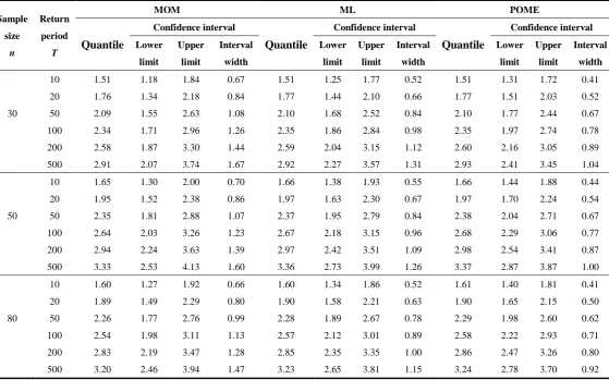
_T corresponding to different

return periods (T=10, 20, 50, 100, 200, and 500) were calculated. Table 1 lists the median values

of the estimated quantiles and confidence intervals by each method.

From Table 1, generally for all cases with sample size n=30, 50, 80, it was observed that

the median of quantiles estimated by the three methods were very close. For example, for the

sample size n=50, the median of quantiles corresponding to the 100-year return period

estimated by MOM, ML and POME are 2.64, 2.67 and 2.68, respectively. Meanwhile,

compared with the results of MOM and ML, the quantiles estimated by POME have the highest

lower limits, the lowest upper limits, and the narrowest confidence intervals. It indicates that

For example, for the case with n=50, the lower limits of 100 years quantile estimators are 2.03,

2.18, and 2.29 when the MOM, ML and POME were used respectively, the corresponding upper

limits are 3.26, 3.15 and 3.06, and the interval widths are 1.23, 0.96 and 0.77. In addition,

generally for all return periods, it can be observed that the confidence intervals of quantile

estimators, including the lower and upper limits and the interval width, decrease with the

increasing sample size n. For example, for n=30, 50 and 80, the median values of interval widths

for a return period of 200 years estimated by POME are 0.89, 0.87 and 0.80, respectively.

Table 1 Median of estimated quantiles and 95% confidence intervals with generated data

Sample size

n

Return period

T

MOM ML POME

Quantile

Confidence interval

Quantile

Confidence interval

Quantile

Confidence interval Lower

limit

Upper limit

Interval width

Lower limit

Upper limit

Interval width

Lower limit

Upper limit

Interval width

10 1.51 1.18 1.84 0.67 1.51 1.25 1.77 0.52 1.51 1.31 1.72 0.41

20 1.76 1.34 2.18 0.84 1.77 1.44 2.10 0.66 1.77 1.51 2.03 0.52

30 50 2.09 1.55 2.63 1.08 2.10 1.68 2.52 0.84 2.10 1.77 2.44 0.67

100 2.34 1.71 2.96 1.26 2.35 1.86 2.84 0.98 2.35 1.97 2.74 0.78

200 2.58 1.87 3.30 1.44 2.59 2.04 3.15 1.12 2.60 2.16 3.05 0.89

500 2.91 2.07 3.74 1.67 2.92 2.27 3.57 1.31 2.93 2.41 3.45 1.04

10 1.65 1.30 2.00 0.70 1.66 1.38 1.93 0.55 1.66 1.44 1.88 0.44

20 1.95 1.52 2.38 0.86 1.97 1.63 2.30 0.67 1.97 1.70 2.24 0.54

50 50 2.35 1.81 2.88 1.07 2.37 1.95 2.79 0.84 2.38 2.04 2.71 0.67

100 2.64 2.03 3.26 1.23 2.67 2.18 3.15 0.96 2.68 2.29 3.06 0.77

200 2.94 2.24 3.63 1.39 2.97 2.42 3.51 1.09 2.98 2.54 3.41 0.87

500 3.33 2.53 4.13 1.60 3.36 2.73 3.99 1.26 3.37 2.87 3.87 1.00

10 1.60 1.27 1.92 0.66 1.60 1.34 1.86 0.52 1.61 1.40 1.81 0.41

20 1.89 1.49 2.29 0.80 1.90 1.58 2.21 0.63 1.90 1.65 2.15 0.50

80 50 2.26 1.77 2.76 0.99 2.28 1.89 2.67 0.78 2.29 1.98 2.60 0.62

100 2.54 1.98 3.11 1.13 2.57 2.12 3.01 0.89 2.58 2.22 2.93 0.71

200 2.83 2.19 3.47 1.28 2.85 2.35 3.35 1.00 2.86 2.47 3.26 0.80

500 3.20 2.46 3.94 1.47 3.23 2.65 3.81 1.15 3.24 2.78 3.70 0.92

Figure 1 shows the median of standard errors of the quantiles estimators. Apparently, for

all return periods, the POME yields the smallest standard errors of the quantile estimators

than that of MOM and ML estimators. Generally for all estimation methods, the standard errors

of quantile estimators show a decreasing trend when the sample size increases from 30 to 80.

Additionally, the decrease in standard errors is relatively smaller when POME was used. This

might imply that the POME is less affected by sample size. Therefore, the performance of the

POME is found to be superior to MOM and ML, and it is more robust since it is less affected

sample size.

Figure 1 Median of standard errors of quantile estimators for sample size n=30, 50 and 80

5

Application

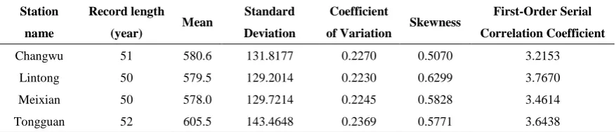
The annual precipitation data from four gauging stations at the Weihe River basin in China

were considered as case study. All data were obtained from the National Climate of China

Meteorological Administration and were complete. The detailed information of these data is

given in Table 2.

Table 2 Basic information on each of the monthly precipitation series used in this study

Station name

Record length

(year) Mean

Standard Deviation

Coefficient

of Variation Skewness

First-Order Serial Correlation Coefficient

Changwu 51 580.6 131.8177 0.2270 0.5070 3.2153

Lintong 50 579.5 129.2014 0.2230 0.6299 3.7670

Meixian 50 578.0 129.7214 0.2245 0.5828 3.4614

Tongguan 52 605.5 143.4648 0.2369 0.5771 3.6438

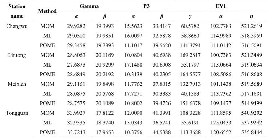
and POME were used to estimate the parameters of these distributions, as given in Table 3. It

can be seen that the parameters of Gamma distribution estimated by MOM, ML and POME are

very close, and so are the EV1 distribution, while those of the P3 distribution depart

significantly.

Table 3 Parameter values of each distribution estimated by the three methods

Station

name Method

Gamma P3 EV1

α β α β γ α u

Changwu MOM 29.9282 19.3993 15.5623 33.4147 60.5782 102.7783 521.2619

ML 29.0510 19.9851 16.0097 32.5878 58.8660 114.9989 518.3959

POME 29.3458 19.7893 11.1017 39.5620 141.3794 111.0142 516.5091

Lintong MOM 28.8063 20.1169 10.0804 40.6938 169.2817 100.7383 521.3449

ML 27.6873 20.9299 17.1488 30.6908 53.1797 113.0664 519.0634

POME 28.6849 20.2192 10.3139 40.2305 164.5577 108.5086 516.8608

Meixian MOM 29.1161 19.8498 11.7762 37.8015 132.7913 101.1438 519.5689 ML 28.0875 20.5768 17.7271 30.3383 40.1383 113.7362 517.1681

POME 28.7575 20.1089 10.8002 39.4726 151.6378 109.1477 514.9499

Tongguan MOM 33.9927 17.8122 12.0090 41.3991 108.3228 111.8595 540.9202

ML 32.9535 18.3740 15.0343 36.5741 55.6191 125.0433 537.9242

POME 33.7243 17.9653 10.3756 44.5388 143.3688 120.6552 535.8444

To evaluate and compare the performance of the three methods and the distributions, the

ordinary least square (OLS) criterion, Akaike information criterion (AIC), and Quasi-optimal

deterministic coefficient test (QD) were employed that can be defined as:

(

)



= −

= n

i xi xi

n OLS

1

2

ˆ 1

(77)

(

x x

)

m n

n

AIC n

i i ˆi 2

1 ln

1

2 ₊

   



 ₋

=



₌ (78)

(

)

(

)





= =

− − −

= _n

i i n

i

i i

x x

x x QD

1

2 1

2

ˆ

1 (79)

where x_i and xˆ_i are the observed data and the predicted values of a given (i-th) quantile,

model, and n is the sample size.

The OLS criterion is recommended as a curve optimization rule for measuring the

difference between empirical and theoretical values in hydrological frequency analysis in China.

The smaller OLS values represent the better performance of the model. The AIC is more

appropriate for the comparison of models have different number of parameters. Given a set of

candidate models for the data, the best model is the one with the minimum AIC value. QD is

used to describe the fitting degree of observed values and theoretical values and the best fit

model is the one that gets the QD value closest to 1. The OLS, AIC, and QD were calculated as

given in Table 4.

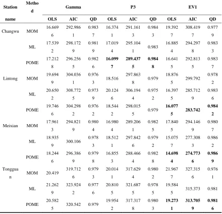
It is seen from Table 4 that the selected best parameter estimation method for each

distribution by the three criterions is coincident and the result of the best fitted distribution for

each station by the three criterions is the same as well. Take the Changwu station in Table 4

for example. According to the smallest OLS and AIC values and the largest QD values, the

POME, MOM and POME are suggested to be the best methods for parameter estimation for

Gamma, P3 and EV1 distributions, respectively. And the best fitted distribution for Changwu

station recommended by the OLS, AIC and QD criteria is P3 distribution. Additionally,

according to the results given in Table 4, the best fitted distributions for the gauging stations

Meixian, Tongguan and Lintong recommended by the OLS, AIC and QD methods, is EV1

distribution with the parameters estimated by POME. Thus the best estimation method for

each station is POME and this is coincident with the results of the simulation experiments in

Section 4, which shows that the performance of POME is better than MOM and ML. The bold

Table 4 OLS, AIC and QD of five distributions for each data series calculated by MOM, ML and POME

Station Metho

d Gamma P3 EV1

name OLS AIC QD OLS AIC QD OLS AIC QD

Changwu MOM 16.669 6

292.986 1

0.983 7

16.374

1

291.161

3

0.984

3

19.392

7

308.419

7

0.977

9

ML 17.539 2

298.172 9

0.981 9

17.019

4

295.104

1 0.983

16.885

4

294.297

8

0.983

3

POME 17.212 8

296.256 5

0.982 6

16.099 7

289.437 5

0.984 8

16.641

5

292.813

5

0.983

7

Lintong MOM 19.694 9

304.036 1

0.976

3 18.516

297.863

8 0.979

18.876

5 299.792 0.978

2

ML 20.650 2

308.772 5

0.973 9

20.124

6

306.194

4

0.975

2

16.397

5

285.712

9

0.983

6

POME 19.746 6

304.298 2

0.976 2

18.544

2

298.015

5 0.979

16.077

5 283.742 0.984

2

Meixian MOM 17.961 3

294.821 9

0.980 4

16.980

4

289.206

1

0.982

5

17.840

5

294.146

9

0.980

7

ML 18.935

9 300.106 0.978

3

18.512

1

297.842

6

0.979

2

15.075

7

277.308

3

0.986

2

POME 18.244 6

296.386 9

0.979 8

16.855

3

288.466

4

0.982

8

14.698 4

274.773 6

0.986 9

Tonggua

n MOM 20.419

319.712 6

0.979 3

20.014

1

317.629

4

0.980

2

21.967

7

327.315

6

0.976

1

ML 21.262 9

323.924 2

0.977 6

20.810

5

321.687

5

0.978

5

19.584

5 315.373 0.981

POME 20.582

5 320.542 0.979

19.954

2

317.317

8

0.980

3

19.273 1

313.705 9

0.981 6

Bold values indicate the smallest OLS and AIC values and the largest QD values.

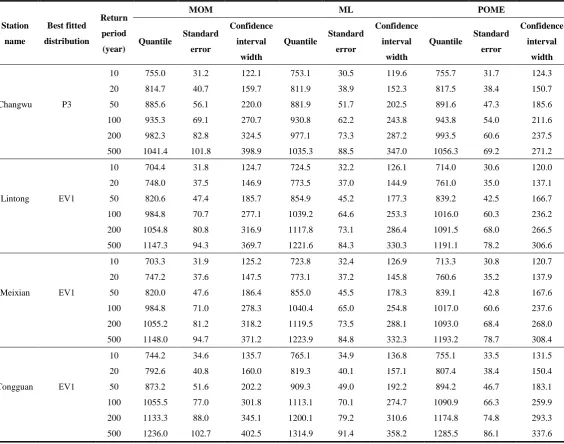
The quantiles along with the standard errors and 95% confidence intervals for 10, 20, 50,

100, 200 and 500 year return periods of the best fitted distribution based on the parameters

estimated by POME are given in Table 5. For the sake of comparison, the quantiles, standard

errors and 95% confidence interval widths based on MOM and ML are also given in Table 5.

The results show that the standard errors and confidence interval widths of quantile estimators

obtained by POME are smaller than those obtained by MOM and ML methods, excepting the

results of T=10 at Changwu station, which indicates that the POME yields more precise

Table 5 Quantile estimators, standard error and 95% confidence interval widths based on MOM, ML and POME for the annual precipitation (mm)

Station name

Best fitted distribution

Return period (year)

MOM ML POME

Quantile Standard error

Confidence interval

width

Quantile Standard error

Confidence interval

width

Quantile Standard error

Confidence interval

width

10 755.0 31.2 122.1 753.1 30.5 119.6 755.7 31.7 124.3

20 814.7 40.7 159.7 811.9 38.9 152.3 817.5 38.4 150.7

Changwu P3 50 885.6 56.1 220.0 881.9 51.7 202.5 891.6 47.3 185.6

100 935.3 69.1 270.7 930.8 62.2 243.8 943.8 54.0 211.6

200 982.3 82.8 324.5 977.1 73.3 287.2 993.5 60.6 237.5

500 1041.4 101.8 398.9 1035.3 88.5 347.0 1056.3 69.2 271.2

10 704.4 31.8 124.7 724.5 32.2 126.1 714.0 30.6 120.0

20 748.0 37.5 146.9 773.5 37.0 144.9 761.0 35.0 137.1

Lintong EV1 50 820.6 47.4 185.7 854.9 45.2 177.3 839.2 42.5 166.7

100 984.8 70.7 277.1 1039.2 64.6 253.3 1016.0 60.3 236.2

200 1054.8 80.8 316.9 1117.8 73.1 286.4 1091.5 68.0 266.5

500 1147.3 94.3 369.7 1221.6 84.3 330.3 1191.1 78.2 306.6

10 703.3 31.9 125.2 723.8 32.4 126.9 713.3 30.8 120.7

20 747.2 37.6 147.5 773.1 37.2 145.8 760.6 35.2 137.9

Meixian EV1 50 820.0 47.6 186.4 855.0 45.5 178.3 839.1 42.8 167.6

100 984.8 71.0 278.3 1040.4 65.0 254.8 1017.0 60.6 237.6

200 1055.2 81.2 318.2 1119.5 73.5 288.1 1093.0 68.4 268.0

500 1148.0 94.7 371.2 1223.9 84.8 332.3 1193.2 78.7 308.4

10 744.2 34.6 135.7 765.1 34.9 136.8 755.1 33.5 131.5

20 792.6 40.8 160.0 819.3 40.1 157.1 807.4 38.4 150.4

Tongguan EV1 50 873.2 51.6 202.2 909.3 49.0 192.2 894.2 46.7 183.1

100 1055.5 77.0 301.8 1113.1 70.1 274.7 1090.9 66.3 259.9

200 1133.3 88.0 345.1 1200.1 79.2 310.6 1174.8 74.8 293.3

500 1236.0 102.7 402.5 1314.9 91.4 358.2 1285.5 86.1 337.6

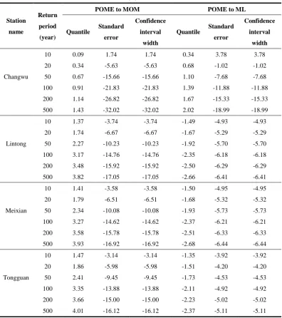
To better understand the performance of the different methods, the differences in the

uncertainty reductions for the standard errors and 95% confidence interval widths of the

quantile estimators were given in terms of relative deviation as shown in Table 6. For the

relatively long return period (T 50), there are significant reductions in the standard errors

and 95% confidence interval widths obtained by POME compared to MOM. For example, for

a return period of T=500, the reductions in standard errors and the confidence interval widths