Performance Analysis of Data–Driven and
Model–Based Control Strategies Applied to a
Thermal Unit Model
Cihan Turhan1, Silvio Simani2,*, Ivan Zajic3and Gulden Gokcen Akkurt4
1 Mechanical Engineering, Izmir Institute of Technology, Gulbahce Campus, Urla, 35430 Izmir, Turkey; [email protected]
2 Dipartimento di Ingegneria, Università degli Studi di Ferrara, Via Saragat 1E, 44122 Ferrara (FE), Italy 3 Control Theory and Applications Centre, Coventry University, CV1 5FB Coventry, UK;
4 Energy Engineering Program, Izmir Institute of Technology, Gulbahce Campus, Urla, 35430 Izmir, Turkey; [email protected]
* Correspondence: [email protected]; Tel.: +39 0532 97 4844
Abstract: The paper presents the design and the implementation of different advanced control strategies that are applied to a nonlinear model of a thermal unit. A data–driven grey–box identification approach provided the physically meaningful nonlinear continuous–time model, which represents the benchmark exploited in this work. The control problem of this thermal unit is important since it constitutes the key element of passive air conditioning systems. The advanced control schemes analysed in this paper are used to regulate the outflow air temperature of the thermal unit by exploiting the inflow air speed, whilst the inflow air temperature is considered as an external disturbance. The reliability and robustness issues of the suggested control methodologies are verified with a Monte–Carlo analysis for simulating modelling uncertainty, disturbance and measurement errors. The achieved results serve to demonstrate the effectiveness and the viable application the suggested control solutions to air conditioning systems. The benchmark model represents one of the key issues of this study, which is exploited for benchmarking different model–based and data–driven advanced control methodologies through extensive simulations. Moreover, this work highlights the main features of the proposed control schemes, while providing practitioners and heating, ventilating and air conditioning engineers with tools to design robust control strategies for air conditioning systems.
Keywords: modelling and simulation for control; advanced control design; model–based and data-driven approaches; artificial intelligence; thermal unit nonlinear system
1. Introduction
solutions. Moreover, the TU module can include nonlinear functions [9], such as products between air temperature and mass flow rate, which can require advanced control strategies to achieve more complex thermal comfort indices and lower energy consumption. To overcome these problems, control strategies relying on Artificial Intelligence (AI) tools, namely Artificial Neural Network (ANN), Fuzzy Logic (FL), Adaptive Neuro-Fuzzy Inference System (ANFIS) and Model Predictive Controllers (MPC) have been proposed to obtain more advanced comfort issues in building applications [10–13]. As an example, a FL control scheme was proposed in [14], where the heat, the humidity, and the oxygen particle concentration represented the control variables, while the fresh air inflow and the fan circulation rate were the monitored outputs. It was shown that FL allowed for more accurate and straightforward results when compared to linear control schemes. A different FL controllers to regulate the air conditioning system temperature was proposed in [15], which was able to easily manage the system nonlinearity.
Other contributions considered different ANN tools that are able to enhance the design of suitable controllers used in air conditioning applications [3,12]. As an example, ANN controllers were proposed in [12] for an air conditioning system, and compared with a standard PID regulator. It was shown how these ANN controllers allowed to achieve a controlled output with a shorter settling time and almost zero overshoot. The main advantage of ANN controllers is represented by their interesting features of automatic learning, easy adaptation, and straightforward generalisation. However, more efficient solutions were proposed, and based on the ANFIS tool [15–18]. In particular, in [15] ANFIS was successfully exploited as alternative control strategy with Heating, Ventilation and Air Conditioning (HVAC) systems to achieve accurate tracking errors.
Other works proposed MPC schemes for the temperature control of buildings [2,19–21]. As an example, in [2] it was shown that the MPC scheme was able to achieve both thermal comfort and energy saving features. Similarly, [19] suggested a more efficient control method when compared with traditional weather–compensated control schemes. Moreover, [22] addressed an interesting overview of MPC methodologies for HVAC systems.
Note that recent studies considered the achievement of thermal comfort and energy efficiency issues using AI tools. However, the performances obtained by these AI based-methods were not analysed in detail and compared via extensive simulations as proposed in this paper using the Monte–Carlo tool. Moreover, this work illustrates the design and the implementation of different control schemes with application to a nonlinear TU dynamic module proposed by the same authors in [9]. Note also that the same authors presented some preliminary results in [23–25], but the analysis of the achievable properties, the robustness features of the proposed solutions with their reliability characteristics have been described in detail in this paper.
Another key issue of the present study consists of illustrating the viable application of the suggested control schemes to real air conditioning systems. This point is fundamental for enhancing practitioners and HVAC young engineers to acquire the fundamentals and the basic design tools for effective HVAC controller development and application. To this aim, the suggested simulations have been synthesised in the MatlabR and SimulinkR environments and exploiting their standard
toolboxes or free software tools. Note that some control strategies proposed in this work were already successfully applied to nonlinear models of energy conversion systems as showne.g.in [26–28].
The remaining of the paper is organised as follows. Section2 provides an overview of the TU module and its mathematical description. Section 3 illustrates the suggested control schemes exploited in this study, whilst the obtained results are reported in Section 4. The reliability and robustness characteristics of the proposed tools in simulation are discussed in Section4.1. Finally, Section5ends the work by summarising the main achievements of the paper. Open problems and future issues that requires further investigations are also suggested.
2. Thermal Unit Mathematical Description
The TU module considered in this study consists of a fundamental block of the whole test–rig proposed for the description and the assessment of the dynamic behaviour of Phase Change Material (PCM) systems used in passive air conditioning plants. Figure1represents the complete PCM system facility considered in [9], where the air flow speed and the temperature are the controlled variables that are exploited to perform the presented simulations and experiments. The heating element included into the PCM system is also sketched.
PCM System Heating Element
(a) (b)
Figure 1.(a) the complete PCM system and (b) the heating element.
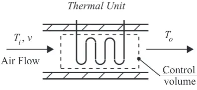
On the other hand, Figure2 illustrates how the inflow air is treated by means of the Heating Element (HE) of the TU. Moreover, the TU module is in a down stream series connection with a cooling unit, which is not reported in Figure2.
Air Flow
Thermal Unit
T
i,
v
T
oControl
volume
Figure 2.The TU module scheme.
signal measurements ofv,Ti andToare acquired from the cross sectional area centre of the supply duct. Note that the inputTi(t)is considered as a disturbance acting on the controlled system.
The mathematical expressions describing the energy balance of the TU module, its air control volume, and the energy balance with respect to the adjacent duct walls have the following form:
Ch d Th(t)
dt = q(t)−(U A)h (Th(t)−To(t)) (1) 0 = (U A)h (Th(t)−To(t))−v(t)ρaAaca (To(t)−Ti(t))−(U A)int (To(t)−Tw(t))(2) Cw d Tw(t)
dt = (U A)int(To(t)−Tw(t))−(U A)ext (Tw(t)−Ta(t)) (3) where the variableCh[J/K] indicates the heating element thermal capacity,Cw[J/K] is the thermal wall capacity (insulated plywood), ca [J/kg K] represents the air specific heat capacity, Aa [m2] is the cross sectional area of the duct,ρa[kg/m3] denotes the air density,q(t)represents the supplied constant heat gain, whilstU[J/m2K] indicates the heat transfer coefficient. Note that in Eqs. (1) – (3), the term (U A)h[J/K] indicates the product of the heat transfer coefficientU[J/m2 K] with the efficient surface area, A[m2], through which the heat is transmitted and regarding the TU module. On the other hand,(U A)int[J/K] indicates the coefficient with reference to the inner duct wall, whilst (U A)ext[J/K] denotes the same term regarding the outer duct wall.
The variablesTh(t)[K],Tw(t)[K] andTa(t)[K] denote the average heating element temperature, the wall temperature and outside air temperature, respectively. Note that the air surrounding the heating element is assumed to be perfectly mixed. Therefore, the outlet air temperature To(t) is equal to the mean temperature of the whole control volume under the lumped parameter modelling approach (see Eq. (1)). Moreover, the thermal capacity of the air passing thought the TU element of Figure2is assumed to be very small so that the heat transfer between the heating element and the air is instantaneous. Under this assumption, the left side of the Eq. (2) is zero. Finally, in Eq. (3) it is assumed that the heat loss occurs only through the walls of the duct.
A standard thermocouple type K has been used to measure the air temperatures. The accuracy is around 1oCfor the whole measurement range. The airflow has been measured using a Hot Wire Thermo–Anemometer with declared accuracy of 5%. For more details regarding the TU module, which is beyond the scope of this paper, the interested reader is referred to [9].
The authors in [9] showed that the complete dynamic behaviour of the TU module is described by a continuous–time time–invariant nonlinear model consisting of a product of two second–order continuous–time time–invariant transfer functions in the form of Eq. (4):
To(t) = ˆ
β1s+βˆ2 s2+αˆ
1s+αˆ2
(Ti(t)v(t)) + ˆ
η1s+ηˆ2 s2+αˆ
1s+αˆ2
(To(t)v(t)) +εˆ (4)
where sdenotes a differential operator. The parameters ˆαi, ˆβi, ˆηi and ˆεof the model in the form
of Eq. (4) were obtained by using a refined instrumental variable method described in [9]. These values are reported in Table1. The model is considered to be of low complexity yet achieving high
Table 1.Estimated model parameters with their accuracy [9].
Parameter αˆ1 αˆ2 βˆ1 βˆ2
Value 55.026±2.011 -92.835±3.398 9.9837±0.2512 7.7661±0.2835
Parameter ηˆ1 ηˆ2 εˆ
Value -8.5689±0.2070 -8.3067±0.2984 -122.95±4.426
the system simulation and improved model–based and data–driven control designs for temperature regulation, as shown in the following sections.
3. Control Designs for the TU Module
With reference to the systems sketched in Figure2, and modelled by the expressions of Eqs. (1) – (3), the general plant can be described as a Multiple–Input Single–Output (MISO) time–invariant nonlinear model, where the input–output air temperatures and its air flow represent the main input–output variables. Its input–output dynamic behaviour can be described as a nonlinear dynamic functionF in the general form of Eq. (5):
y(t) =F(u(t),t) (5)
wherey(t)is the output variable,i.e. To(t),u(t)is the input vector,i.e.[Ti(t),v(t)]Tandtis the time. The control law designed to be applied to the TU module in general determines the control input injected into the controlled plant of Eq. (5) in order to track a given reference, or set–point, denoted asr(t).
It is worth observing that the design and the performance of control systems for generic TU processes are strongly determined by the bilinear terms represented in Eq. (4), where the nonlinear behaviour is described by the product between the air temperature and its mass flow rate. Under this consideration, in order to enhance the control law designs and their implementation, the inlet air temperature Ti(t)is considered as a measurable disturbanced(t). The input–output data acquired from the test–rig and the TU module in Figures1and2are represented by the inlet air temperature Ti(t), the air flowv(t), and the outlet air temperatureTo(t).
In the remainder of this section, different control laws and their implementations are summarised. The methods include the standard PID regulator, and nonlinear control methodologies relying on AI techniques, such as FL and adaptive schemes, as well as the model predictive control. These control strategies, that are exploited for the the regulation of the outlet air temperatureTo(t), will be applied to the TU system of Figure2described by the model of Eq. (4).
3.1. Standard PID Controller Design
Several works [5–7,12,30] highlighted that standard PID controllers can be commonly used in general HVAC applications. In fact, it is shown that simple PID controllers are able to achieved interesting results based on the direct and straightforward computation of the tracking error e(t) computed as difference between the reference and the measured values of the output, respectively,i.e. e(t) =r(t)−y(t). The continuous–time standard PID controller can be represented in the following parallel form [31,32]:
u(t) =Kp+Ki
Z t
0 e(τ)dτ +Kd
de(t)
dt (6)
where Kp, Ki, and Kd are the PID proportional, integral and derivative gains, respectively. Note that the derivative term of the PID controller is usually implemented as first order filter whose pole location is defined by the coefficientTf. The derivation of the PID gains when this standard controller is applied to the TU module of Section 2 will be achieved by means of the auto–tuning approach proposede.g.in [32] and implemented in the MatlabR environment.
3.2. Fuzzy Controller Design
According to this description, the TS fuzzy prototype relies on a suitable number of rules denoted asRi, where the consequent terms are deterministic functions in the form of fi(.). The subscripti indicates thei–th rule, which is usually represented in the form of:
Ri: IF x∈Ai THEN yi= fi(x) (7)
wherei=1, 2, . . . ,K, andKrepresents a suitable number of rules. In Eq. (7) the variablexindicates the antecedent terms, whilst the scalaryi represents the consequent output. For thei–th rule, the fuzzy set Ai is represented in general by a multivariable membership functionµAi(.)described by the relation of Eq. (8) [39]:
µAi(x): Ai(x)7→[0, 1] (8)
The consequent functions fi(.)can be represented by parametric models, with fixed structure and varying parameters, as addressed by the same authorse.g.in [40]. The function fi(.)can be described with a suitable parameterisation in affine form, and usually represented in the form of Eq. (9):
yi=aTi x+bi (9)
where the model parameters are the column vectorai and the scalarbi, for a number of rulesi = 1, 2, . . . ,K. The variable x is a column vector consisting of an appropriate numbern of delayed samples of the input and output signalsu(t)and y(t)acquired from the controlled process. Under this description, the termaiTxrepresents a linear regression [42].
It is important to note that the prototypes in the form of Eq. (7) have interesting approximation properties [41]. In fact, if the consequents functions fi(.)are represented in the form of Eq. (10) [42]:
Ri: IF x∈ Ai THEN yi(tk) = n
∑
j=1
α(ji)y(tk−T j) + n
∑
j=1
β(ji)u(tk−T j) +bi (10)
the collection of the systems of Eq. (10) can approximate the dynamic behaviour of any process with an accuracy depending on the choice of the structure. tk is the time sample T k corresponding to the sampling time T. According to this description, n represents the order of the regression model, the antecedents depends on the column vector x = x(tk) = [y(tk−T), . . . ,y(tk−T n),u(tk−T), . . . ,u(tk−T n)]T, whilst the consequents are affine with parameter vectorai=
h
α1(i), . . . , α(ni),β(1i), . . . , β(ni)
iT
and scalarbi.
It is worth noting that the complete behaviour of the discrete–time TS fuzzy prototype of Eq. (7), whose output isycan be expressed in the form of Eq. (11):
y= ∑ K
i=1µAi(x)yi(x)
∑K
i=1µAi(x)
(11)
According to this representation, this work proposes to use the TS fuzzy model as prototype for providing the mathematical description of the controller exploited for the compensation of the TU module of Section2. The estimation of the structure of the model of Eq. (11) can be obtained by means of the ANFIS tool relying on the following steps [38]:
1. A TS prototype structure with order n, the membership functions µAi(.), and an appropriate number of rulesKare assumed;
2. The input and output data sampled from the process under control are exploited by ANFIS tool for providing the TS model parametersaiandbiaccording to a selected error criterion;
This study proposes also a different methodology based on the Fuzzy Modelling and Identification (FMID) toolbox developed in the MatlabR environment [43]. This tool allows to obtain in an easy
and straightforward way the parameters of the TS fuzzy structure of Eq. (11). Moreover, the FMID strategy provides the controller model simply using a data–driven approach scheme addressed in [43]. This approach exploits again the estimation of the rule–based fuzzy model parameters and requires only the input–output data sampled from the controlled process. In particular, the FMID scheme uses the Gustafson–Kessel clustering methodology to partition the input–output data into suitable regions, denoted again asRi, the so–called clusters [43]. For eachi–th cluster, the parameters ai and bi of the affine models of Eq. (9) with their membership functionµAi(.)are derived. The estimation of the TS fuzzy model in the form of Eq. (11) is based on the choice of a suitable model structurenand a number of rulesK(usually equal to the number of clusters). The selection of these parameters is performed in order to minimise a prescribed cost function usually related with the closed–loop system performance [43].
In this way, the FMID approach estimates the parametersai,bi and the membership functions
µAi(.). Moreover, this strategy is exploited again for identifying the mathematical description of the fuzzy controller that minimises a suitable cost function of the tracking errore(t). Note finally that the FL controller in the form of Eq. (11) is implemented as discrete–time model that will be connected to the TU process of Eq. (4) via suitable Digital–to–Analog (D/A) and Analog–to–Digital (A/D) converter devices [31].
3.3. Adaptive Controller Design
This study proposes the derivation of the controller model for the regulation of the TU module of Section2by means of an adaptive strategy. This on–line approach relies on the recursive identification of second order discrete–time in its difference form of Eq. (12):
y(tk) =βˆ1u(tk−1) +βˆ2u(tk−2)−αˆ1y(tk−1)−αˆ2y(tk−2) (12)
where its time–varying parameters ˆαiand ˆβiare recursively identified at each sampling timetk=k T, withkthe sample index (k=1, . . . ,N, andNthe total number of samples) andTthe sampling time. This adaptive identification mechanism uses Recursive Least Squares Method (RLSM) with adaptive directional forgetting as described in [44], since it is already implemented and ready to use in the SimulinkR environment [45].
Under this assumption, the adaptive controller design approach exploits a modified Ziegler–Nichols method that is used to achieve the control law in the form of Eq. (13) [44]:
u(tk) =q0e(tk) +q1e(tk−T) +q2e(tk−2T) + (1−γ)u(tk−T) +γu(tk−2T) (13) wheree(tk)is the tracking error at the instanttk=k Tandu(tk)is the control signal at the sampling timek T. The variablesq0,q1,q2, andγin Eq. (13) represent the time–varying controller parameters,
which are obtained by solving the Diophantine expressions represented in the form of Eqs. (14) [44]:
q0 = βˆ11 (d1+1−αˆ1−γ) q1 = αβˆˆ22 −q2
ˆ
β1 ˆ
β2 − ˆ
α1 ˆ
α2 +1
(14)
where the following relations hold:
γ = q2
ˆ
β2 ˆ
α2 q2 =
ˆ
α2((βˆ1+βˆ2) (αˆ1βˆ2−ˆα2βˆ1)+βˆ2(βˆ1d2−βˆ2d1−βˆ2))
(βˆ1+βˆ2) (αˆ1βˆ1βˆ2−αˆ2βˆ21−βˆ22)
It is worth noting that the dominant poles of the controlled system can be represented via the characteristic polynomial in the form of Eq. (16):
s2+2δ ωns+ω2n (16)
where the variables δ and ωn indicate the damping factor and the resonant natural frequency, respectively. Therefore, they can be used for computing adaptive controller parameters in Eq. (13) since these relations are already available from the Digital Self-Tuning Controller (DSTC) toolbox implemented in the MatlabR and SimulinkR environments [45].
Note finally that the difference equation of Eq. (13) represents a discrete–time control law that requires suitable D/A and A/D converters to be applied to the continuous–time TU model of Eq. (4) in Section2. Therefore, with reference to Eq. (13), the tracking errore(tk)is computed as the difference between the sampled reference signalr(tk)and the sampled controlled outputy(tk). 3.4. Model Predictive Controller Designs
The regulation strategy relying on the Model Predictive Controller (MPC) method exploits the reconstruction of the system outputy(tk)for a number of step–ahead predictions,i.e. the so–called prediction horizon, in order to generate a suitable control sequence u(tk) [46]. This methodology provides the control law at the current sampling timetk=k T, once it has been derived and optimised over a suitable and finite time horizon. One of the most important features of the MPC scheme with respect to standard PID control relies on its ability to anticipate future behaviours, thus taking the required control actions accordingly. An example of application of MPC to HVAC systems is shown e.g.in [22] and compared with other control approaches. However, this work analyses viable control solutions with application to both the simulated and real system, in order to highlight advantages and drawbacks of the suggested solutions.
In more detail, the MPC scheme generates a suitable control signalu(tk) by performing the minimisation of the cost function in the form of Eq. (17) [46]:
J= Np
∑
k=1
wyk (r(tk)−y(tk)) + Nc
∑
k=1 wuk∆u
2(t
k) (17)
with wyk representing suitable weighting parameters indicating the relative importance of the sampled controlled outputy(tk)with respect to the sampled reference r(tk). In the same way, the coefficientswukrepresent weighting factors penalising possible variations of the actual control signal u(tk) at the instant k T with respect to its previous value at the sampling time tk−1 = (k−1)T, i.e. ∆u(tk) = u(tk)−u(tk−1). Moreover, the cost function depends on appropriate values of the
prediction horizonNpand the control horizonNc.
With this approach, by minimising the expression of Eq. (17), the MPC strategy generates and applies only the first elementu(tk)of the whole control sequence at the time sampletk, whilst the future values of the sequence are dropped. On the other hand, at the next time instant tk+1, the
controlled outputy(tk+1)is measured, and the new control law is computed, thus generating a new
control vectoru(tk+1)and its prediction sequence. This approach is recursively iterated in order to
perform the complete simulation of the controlled system.
It is worth observing that the discrete–time MPC design is achieved in a straightforward way by exploiting the MPC toolbox in the SimulinkR environment, which can require the knowledge of
a state–space LTI model of the controlled process of Eqs. (4). A continuous–time LTI description of this dynamic process can be obtained by means of the linearisation of Eq. (4), which leads to the state–space model in the form of Eq. (18):
(
˙
x(t) = Ax(t) +Bu(t)
where x(t) ∈ <4 represents the state vector, whilst the state–space model matrices A, B, and
C are defined by the linearisation at the operating point corresponding to the equilibrium state xe =1.0093×10⁵, 444.3758, −87436, −0.6288Tand inputsue= [19.2351, 0.9093]T:
A=
−0.0550 0.0001 0 0
1.0000 0 0 0
0.0908 0.0007 −0.1329 −0.0007
0 0 1.0000 0
, B= 0.9093 19.2351 0 0
0 −122.9626
0 0
, C= 0.0998 0.0008 −0.0857 −0.0008 T (19) With reference to the system in Figure2, the air flow velocityv(t)represents the control input,y(t) = To(t)is the controlled output of the model of Eq. (18), whilstTi(t)is the measurable disturbanced(t). Therefore, the input vector in Eq. (18) isu(t) = [Ti(t),v(t)]T.
Note that the discrete–time MPC design is achieved by using the MPC toolbox in the SimulinkR
environment, which uses a state–space LTI description of the controlled process of Eqs. (4). A continuous–time model of this plant can be obtained by means of an identification procedure, for example based on the System Identification Toolbox in the MatlabR environment. In this way, the
subspace identification (N4SID) procedure has lead to the state–space matrices in Eqs. (20) [42]:
A=
0.005791 −0.03346 0.06669 0.03293
−0.03849 −0.8226 3.345 1.513 0.03747 1.386 −6.579 −2.869
−0.1521 −1.89 7.195 2.452
, B=
−0.2953 0.01477
−13.28 0.9604 25.28 −1.923
−23.73 1.783
, C= 84.4 −0.8255 0.1243 0.118 T (20) for a state–space model that is able to fit the identification data with an accuracy higher than 76% [42]. Similar procedures were proposede.g.in [47,48].
Note also that the MPC design can be performed also directly exploiting nonlinear formulations. In fact, this control package accepts also nonlinear models. In particular, using large–scale nonlinear programming solvers such as Advanced Process OPTimizer (APOPT) and Interior Point OPTimizer (IPOPT) , which are available in the Optimization Toolbox in the MatlabR and SimulinkR
environments. Therefore, this simulation code is able to implement the moving horizon estimation, dynamic optimisation and simulation, thus solving the nonlinear MPC problems [29]. The nonlinear input–output dynamic model used in simulation has been obtained again by exploiting the System Identification Toolbox in the MatlabR environment. In particular, this estimation procedure
performed via a Prediction Error Method (PEM) has provided a nonlinear regression model with 2 inputs and 1 output, with standard regressors corresponding to the ordersna = nb = 2 for both the inputs and the output, without dead–times (nk = 1) [42]. Moreover, the nonlinearity has been modelled via a sigmoidal network with 10 neurons. Therefore, this nonlinear regression model is able to fit the identification data with an accuracy higher than 90% [42]. Section 4 will show and compare the results achieved with the different models implementing both the linear and nonlinear MPC strategies.
Finally, also in this case the discrete–time regulators obtained via the MPC approach are connected to the continuous–time TU system via D/A and A/D devices.
4. Simulation Results
The control strategies summarised in Section 3 were applied to the simulated TU process of Eq. (4). The achieved results shown in this section have been obtained in the MatlabR and
will be compared in terms of a performance index represented by the Mean Sum of Squared Error (MSSE%) computed via Eq. (21):
MSSE%=100
v u u t∑
N
k=0(r(tk)−y(tk))2
∑N
k=0r2(tk)
(21)
whereNis the total number of samples.
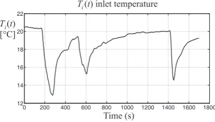
As already remarked, many HVAC systems are controlled via standard PID regulators. Therefore, the first results are achieved by exploiting a regulator in the form of Eq. (6) applied to the TU simulated model as represented in Figure3. Note that in the scheme of Figure3, the control inputu(t)is the inlet air speedv(t), whilst the inlet air temperatureTi(t)is considered asmeasurable disturbanced(t), which is shown in Figure4.
+_
TU simulated
model r(t)
u(t)
y(t)
v(t) Ti d(t)
To
e(t)
y(t)
PID parameter optimiser
System linearised model
PID automatic tuning Simulink toolbox
PI controller
Figure 3.Block diagram of the TU simulator with the standard PID controller.
Time (s) T ti( )
[°C]
0 200 400 600 800 1000 1200 1400 1600 1800 12
14 16 18 20 22
T t( ) inlet temperature i
Figure 4. The inflow air temperatureTi(t)considered as a disturbanced(t)acting on the controlled
system.
With reference to this control strategy, the optimal controller gains are computed using the automatic PID tuning procedure from the PID SimulinkR block. The proportional, integral, and
derivative gains have been determined asKp = 1.4465,Ki = 0.0339, andKd = 0.4228, respectively. The derivative filter coefficient has been estimated asTf =4.4034.
Figure 5 represents the set–point r(t) (blue continuous line) and the TU measured output y(t) = To (red dashed line) regulated via the PID standard controller. With this methodology, the PID regulator is able to guarantee a response with settling timeTs =2.17sand maximum overshoot S% =36.14%. These values are derived by applying a step change in the reference signalr(t)from 39oCto 40oC. The tracking error evaluated via Eq. (21) isMSSE%=1.65%.
0 200 400 600 800 1000 1200 1400 1600 1800 20
40
Time (s)
Reference
PID contr. 25
30 35
To outlet temperature
[°C]
r
y
(t) &
(t)
Figure 5. Controlled outlet temperature To with the PID regulator obtained via the auto–tuning
procedure.
described in [9]. Moreover, the authors have exploited this reference signal since it guarantees the correct working conditions and the validity of the identified model of Eq. (4).
It is worth observing that PID standard controllers can provide sufficient robustness properties after a straightforward tuning phase, thus representing interesting and easy to use solutions with simple and viable implementation. However, in despite of these features, the achieved control laws might not be sufficiently efficient in termse.g.of energy consumption and maintenance costs, when applied to HVAC systems. Due to these possible limitations, the paper has investigated alternative control strategies for achieving improved performances. To this aim, the PID regulator obtained via the auto–tuning procedure is regarded as reference controller for the computation of advanced and alternative control strategies.
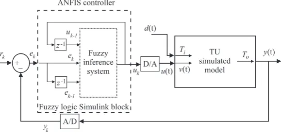
First, a TS fuzzy model of the controller has been derived using the fuzzy identification method recalled in Section 3.2. The procedure exploited the so–called Model Reference Control (MRC) approach describede.g. in [49]. In this way, the TS fuzzy controller is derived via the ANFIS tool, with a sampling intervalT=0.1s.
Figure6 reports the diagram of this control solution, where this fuzzy regulator uses K = 3 Gaussian membership functions and a number of delayed input and output samplesn =1. Figure 6highlights also that the antecedent vector of the ANFIS tool isx(k) = [e(tk),e(tk−1),u(tk−1)]T = [ek,ek−1,uk−1]T.
On the other hand, Figure7reports the achieved performance of the regulator obtained with the ANFIS tool by comparing the referencer(t)(continuous blue line) and controlled outputy(t)(red dashed line). In this case, the settling time isTs =2.21s, with a maximum overshootS%= 38.22% andMSSE%=1.07%.
+_
TU simulated
model
r
u(t)
y(t)
v(t)
Ti d(t)
To
D/A
A/D
y
uk
k
Fuzzy inference
system
z-1 uk-1
k ek
z-1 ek-1
ANFIS controller
ek
Fuzzy logic Simulink block
0 200 400 600 800 1000 1200 1400 1600 1800 24
28 32 36 40
Time (s)
To outlet temperature
[°C]
r
y
(t) &
(t)
Reference
ANFIS
Figure 7.Outlet temperature regulated by the fuzzy controller achieved via the ANFIS tool.
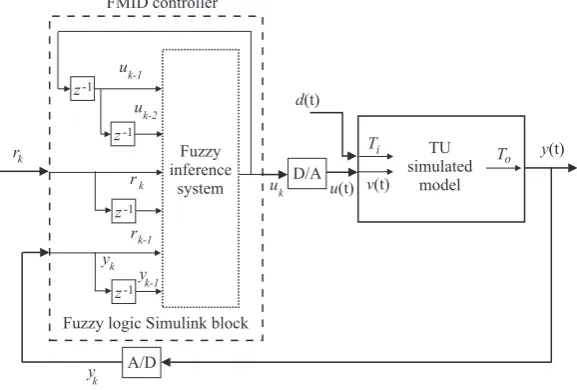
This work also proposes the derivation of a fuzzy controller in form of Eq. (11), whose structure and parameter estimation relies on the FMID tool. This tool is able also to provide the estimation of the fuzzy membership functionsµAi(.)in Eq. (11).
Once the structure of this TS fuzzy regulator has been achieved, the obtained regulator is sketched in Figure8, for an optimal number of clusters K = 3 and delays n = 2. For this fuzzy system, the antecedent vector is defined asx(tk) = [u(tk−1),u(tk−2),r(tk),r(tk−1),y(tk),y(tk−1)]T = [uk−1,uk−2,rk,rk−1,yk,yk−1]T.
TU simulated
model r
u(t)
y(t)
v(t) Ti d(t)
To D/A
A/D y
uk
k
Fuzzy inference
system z-1
uk-2
k
z-1
k-1 FMID controller
rk
z-1 yk-1 r
yk z-1
uk-1
Fuzzy logic Simulink block
Figure 8.Diagram of the TU module with the TS fuzzy regulator identified from the FMID toolbox.
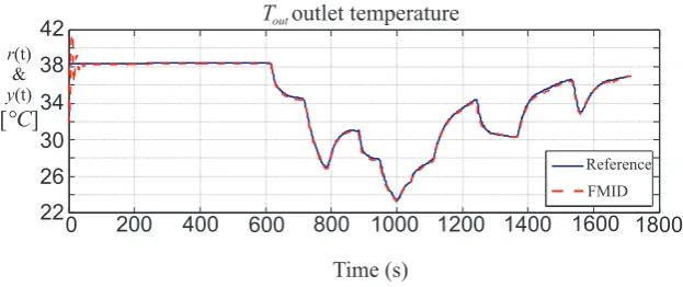
The results achieved by this TS fuzzy regulator obtained via FMID library of the MatlabR
environment are summarised in Figure9. In this situation, the set-pointr(t)(blue continuous line) is tracked with aMSSE%= 1.14%. On the other hand, the step transient response presents a settling timeTs = 3.98sand a maximum overshootS%= 41.65%. Finally, it is worth nothing that the high overshoot at the beginning of the simulation in Figure9is due to the initial conditions of the delay blocks of the fuzzy controller represented in Figure9that are zero.
A further class of regulators has been considered in this work, and an adaptive controller has been developed according to the strategy recalled in Section3.3.
0 200 400 600 800 1000 1200 1400 1600 1800 22
26 38 42
Time (s) Toutoutlet temperature
[°C]
r
y (t) &
(t)
Reference
FMID 30
34
Figure 9.TU outflow air temperature with the TS fuzzy regulator derived via the FMID toolbox.
Eq. (16), which represent the damping factor and the natural resonance frequency of the closed–loop controlled system.
TU simulated
system
r u(t)
y(t)
v(t) Ti d(t)
To D/A
A/D y
u
k
k
z-1 u
k-1
k
u
k
Adaptive controller
Adaptive controller design ARX on-line identification
y
k
r
k
uk-1
u
k
y
k
ai,bi
STCSL Simulink block
Figure 10.Diagram of the TU module controlled by the adaptive regulator.
The tracking performances of the designed adaptive controller are summarised Figure11. In particular, the settling time of the step transient response isTs = 3.65swith a maximum overshoot S%=40.18%, whilst the achieved tracking error corresponds to aMSSE%=1.18%.
0 200 400 600 800 1000 1200 1400 1600 1800
22 26 30 34 38
To outlet temperature
Time (s) [°C]
r
y
(t) &
(t)
Reference
Adaptive
Figure 11.TU module outlet air temperature compensated by the adaptive regulator.
TU simulated
system
r
u(t)
y(t)
v(t)
Ti d(t)
To D/A
A/D
uk
y
k k
dk
MPC controller
Dynamic optimiser
Cost function
System model
MPC Simulink toolbox
A/D
d(t)
Figure 12.Diagram of the TU system controlled by the MPC scheme.
It is worth noting that in this case the MPC design exploits a prediction horizon ofNp=10 and a control horizon ofNc = 2 for the minimisation of the cost function Jof Eq. (17). Moreover, the weighting coefficients of this cost functionJare settled towyk =0.1 andwuk =1 in order to minimise possible abrupt changes of the control inputu(tk)that would increase the energy consumption and the controlled system efficiency.
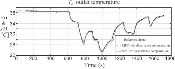
In this situation, as shown in Figure13, the step transient response of the controlled TU module presents a settling timeTs = 1.85sand a maximum overshoot S% = 35.51%, with a tracking error MSSE%=0.41%. Figure13shows also the results obtained with the MPC control using the linearised state–space model of Eq. (19), when the disturbanced(t)does not feed the MPC block of Figure12.
0 200 400 600 800 1000 1200 1400 1600 1800
22 26 30 34 38
Time (s) To outlet temperature
[°C]
r
y
(t) &
(t)
Reference signal
MPC with disturbance compensation
MPC w/o disturbance compensation
Figure 13. TU module outlet air temperature compensated by the linear MPC with and without disturbanced(t)compensation.
Figure13highlights that the knowledge of the measured disturbance d(t)that is exploited by the MPC block of Figure12improves the performance of the linear MPC strategy.
On the other hand, Figure14shows the comparison between the MPC design performed using the identified state–space model of Eq. (20) and the nonlinear dynamic MPC scheme relying on a neural model of the controlled process sketched in Section3.4.
Figure14highlights that the nonlinear MPC leads to slightly better results with respect to the linear MPC with the identified state–space model of Eq. (20).
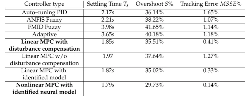
In order to analyse the obtained performance and compare the results achieved with the application of the control strategies proposed in this work, Table2summarises the features of these regulators in terms of step response settling time Ts, maximum overshoot S%, and tracking error MSSE%.
0 200 400 600 800 1000 1200 1400 1600 1800 22
26 30 34 38
Time (s)
To outlet temperature
[°C]
r
y
(t) &
(t)
Reference signal
Linear ident. MPC ctrl. Nonlinear MPC ctrl.
Figure 14.TU module outlet air temperature compensated by the identified linear and the nonlinear MPC solutions.
Table 2.Performances with the proposed controllers.
Controller type Settling TimeTs OvershootS% Tracking ErrorMSSE%
Auto–tuning PID 2.17s 36.14% 1.65%
ANFIS Fuzzy 2.21s 38.22% 1.07%
FMID Fuzzy 3.98s 41.65% 1.14%
Adaptive 3.65s 40.18% 1.18%
Linear MPC with 1.85s 35.51% 0.41%
disturbance compensation
Linear MPC w/o 1.97 37.64% 1.27%
disturbance compensation
Linear MPC with 1.82s 35.02% 0.33%
identified model
Nonlinear MPC with 1.79s 29.73% 0.14%
identified neural model
the ability of the MPC methodology to anticipate future events, thus being able to take control actions accordingly. Moreover, the benefits of exploiting both an identified state–space model and a nonlinear prototype of the controlled process in connection with the knowledge of the measured disturbance d(t)seem quite clear from the results reported in Table2.
On the other hand, also the TS fuzzy controller derived via the ANFIS toolbox in connection with the MRC principle seems to present interesting features in terms of step response settling time, maximum overshoot and tracking error when compared to the other methodologies. This property can be due to the ANFIS strategy that relies on a fuzzy inference system. In fact, the ANFIS scheme includes the capabilities of both the neural network and the fuzzy logic tools, with the advantage of integrating their benefits in one whole structure. Moreover, as already observed, the proposed fuzzy approach that integrates learning capability is able to approximate the process nonlinear behaviour with an error depending on the required accuracy level. The adaptation strategy implemented in ANFIS presents interesting computationally efficient features since it relies on genetic algorithms used to estimate the best model structure and its parameters [49].
Note however that the standard PID regulator leads to achieve the second best step response settling time since it exploits the auto–tuning scheme implemented in the SimulinkR PID block
parameters allows the PID controller to manage general control requirements, also in terms of step response rise time, closed–loop bandwidth, maximum overshoot, and system oscillation amplitude. On the other hand, PID controllers cannot guarantee any control optimality, and in some situations the overall system stability, but provides a viable and easy–to–use tool for providing a simple control law with acceptable performance.
4.1. Control Solution Sensitivity Evaluation
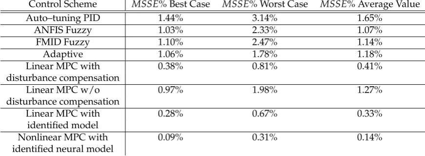
This study has considered further simulations that are useful for analysing the reliability and robustness characteristics of the considered control solutions with respect to possible parameter variations. This approach represents a way for analysing the well–known model–reality mismatch issue that can represent a limitation of the achievable performance of the proposed controller designs. To this aim, the Monte–Carlo (MC) tool is the key point since the controller behaviour and the design strategy depend on this model–reality mismatch, which can derivee.g. from the model nonlinearity and its approximation, the uncertainty and disturbance terms, as well as input and output measurement errors. Therefore, the MC analysis simulates the behaviour of the controlled TU model when its parameters are described as Gaussian variables with mean values equal to the nominal ones, and standard deviations of±20% of the corresponding parameter values.
Under these assumptions, the analysis of the closed–loop control schemes has been performed by computing the best, average, and the worst values of theMSSE% index of Eq. (21) evaluated over 500 MC runs. These values are summarised in Table3.
Table 3.MSSE% values obtained via the MC analysis for controller performance evaluation.
Control Scheme MSSE% Best Case MSSE% Worst Case MSSE% Average Value
Auto–tuning PID 1.44% 3.14% 1.65%
ANFIS Fuzzy 1.03% 2.33% 1.07%
FMID Fuzzy 1.10% 2.47% 1.14%
Adaptive 1.06% 1.78% 1.18%
Linear MPC with 0.38% 0.81% 0.41%
disturbance compensation
Linear MPC w/o 0.97% 1.98% 1.27%
disturbance compensation
Linear MPC with 0.28% 0.67% 0.33%
identified model
Nonlinear MPC with 0.09% 0.31% 0.14%
identified neural model
On the basis of the results of Table 3, it seems clear that the MPC designs lead to the best performance when the modelling of the controlled system and the measured disturbanced(t) =Ti(t) is taken into account. On one hand, the MPC design can rely on the knowledge of a state–space model in the form of Eq. (18), derived from both a linearisation procedure or an identification experiment. On the other hand, the MPC design can use an identified nonlinear model of the process, as remarked at the end of Section3.4. The overall methodology is based on the optimisation of the cost function of Eq. (17). However, once the description of the controlled process has been available as both linear or nonlinear dynamic model, the MPC design is quite simple and straightforward.
The control schemes relying on the ANFIS and the FMID tools can lead to interesting control performance, but with a learning phase that can be computationally heavy and time–consuming, especially when the number of rulesK, the antecedents and the model delaysnare high.
Standard PID regulators require simple design and simple implementation, but in general they lead to limited performance, which can imply lower efficiency when appliede.g. to HVAC systems. The same remarks are valid for the fuzzy controllers relying on AI tools, whose parameters can be easily estimated from the input–output data acquired from the controlled process. However, a further optimisation stage can be required, which sometimes is time–consuming, but these fuzzy solutions can enhance the achievement of advanced performance indices.
It is worth observing that the MC methodology proposed in this work seems to represent the key point for the validation and the verification of the proposed control solutions when applied to the TU module in the presence of modelling and measurement errors, uncertainty and disturbance terms.
Note finally that the control methodologies followed by the analysis procedures shown in Sections3and4are developed using the MatlabR and SimulinkR software tools, in order to automate
the overall design and simulation phases. These feasibility and reliability studies are of paramount importance for real application of control strategies once implemented to future air conditioning system installations.
5. Conclusion
In this work, several data–driven and model–based control strategies were recalled, designed and applied to a nonlinear thermal unit model, which can be considered as a fundamental module of phase change material larger systems exploited in passive air conditioning devices. The feasibility of the obtained solutions and the reliability features of the proposed methodologies were analysed in simulation using the measurements acquired from a realistic test–rig of a passive air conditioning system. The Monte–Carlo tool represented the practical method for validating the features of these control schemes in the presence of modelling, disturbance and measurement errors. The achieved results highlighted that the controllers designed for example with artificial intelligence schemes were able to provide interesting behaviour in terms of settling time, maximum overshoot and tracking error, even if the adaptation phase can be time–consuming. Optimal results were obtained using the model predictive control methodology, even if the derivation of appropriate descriptions of the controlled process and the minimisation of a cost function are required. Finally, future works will investigate the control design and its application for the regulation of different comfort and health parameters of real air conditioning systems, such as the relative humidity, since they directly affect the air conditioning system operating costs in terms of energy.
Author Contributions:Cihan Turhan and Silvio Simani conceived and designed the simulations; Ivan Zajic and Gulden Gokcen Akkurt analysed the methodologies and the achieved results; Silvio Simani wrote the paper.
Conflicts of Interest:The authors declare no conflict of interest.
References
1. Payam, N.; Fatemeh, J.; Mohammad, M.T.; Mohammad, G.; Muhd Zaimi, M.A. A global review of energy consumption, CO2 emissions and policy in the residential sector (with an overview of the top ten CO2 emitting countries). Renewable and Sustainable Energy Reviews 2015, 43, 843–862. DOI: 10.1016/j.rser.2014.11.066.
2. Lindelof, D.; Afshari, H.; Alisafaee, M.; Biswas, J.; Caban, M.; Mocellin, X.; Viaene, J. Field tests of an adaptive, model–predictive heating controller for residential buildings. Energy and Buildings 2015, 99, 292–302. DOI: 10.1016/j.enbuild.2015.04.029.
3. Ferreira, P.M.; Ruano, A.E.; Silva, S.; Conceicao, E.Z.E. Neural networks based predictive control for thermal comfort and energy savings in buildings. Energy and Buildings 2012, 55, 238–251. DOI: 10.1016/j.enbuild.2012.08.002.
5. Mirinejad, H.; Sadati, S.H.; Ghasemian, M.; Torab, H. Control techniques in Heating, Ventilating and Air Conditioning (HVAC) systems.Journal of Computer Science2008,4, 777–783. DOI: 10.3844/jcssp.2008.777.783. 6. Wang, Q.G.; Lee, T.H.; Fung, H.W.; Bi, Q.; Zhang, Y. PID tuning for improved performance.IEEE Transactions
Control System Technology1999,7, 457–465. DOI: 10.1109/87.772161.
7. Rahmati, A.; Rashidi, F.; Rashidi, M. A hybrid fuzzy logic and PID controller for control of nonlinear HVAC systems. Proc. of the IEEE International Conference on Systems, Man and Cybernetics. IEEE, 2003, Vol. 3, pp. 2249–2254. DOI: 10.1109/ICSMC.2003.1244218.
8. Wenqi, G.; Mengchu, Z. Technologies toward thermal comfort–based and energy–efficient HVAC systems: A review. Proc. of the IEEE International Conference on Systems, Man and Cybernetics – SMC 2009. IEEE, 2009, pp. 3883–3888. DOI: 10.1109/ICSMC.2009.5346631.
9. Zajic, I.; Iten, M.; Burnham, K.J. Modelling and data–based identification of heating element in continuous–time domain. Journal of Physics: Conference Series 2014, 570, 012003. DOI: 10.1088/1742-6596/570/1/012003.
10. Krarti, M. An overview of artificial intelligence–based methods for building energy systems.Journal of Solar Energy Engineering2003,125, 331–342. DOI: 10.1115/1.1592186.
11. He, M.; Cai, W.J.; Li, S.Y. Multiple fuzzy model–based temperature predictive control for HVAC systems. Information Science2005,169, 155–174. DOI: 10.1016/j.ins.2004.02.016.
12. Kumar, P.; Singh, K.P. Comparative Analysis of Air Conditional System Using PID and Neural Network Controller. International Journal of Scientific and Research Publications2013,3, 1–6. ISSN: 2250–3153. DOI: 10.1.1.415.2205.
13. Dounis, A.I.; Caraiscos, C. Advanced control systems engineering for energy and comfort management in a building environment – A review. Renewable and Sustainable Energy Reviews2009,13, 1246–1261. DOI: 10.1016/j.rser.2008.09.015.
14. Etik, N.; Allahverdi, N.; Sert, I.U.; Saritas, I. Fuzzy expert system design for operating room air–condition control systems. Expert Systems with Applications2009,36, 9753–9758. DOI: 10.1016/j.eswa.2009.02.028. 15. Soyguder, S.; Alli, H. An expert system for the humidity and temperature control in HVAC systems using
ANFIS and optimization with Fuzzy Modelling Approach. Energy and Buildings2009,41, 814–822. DOI: 10.1016/j.enbuild.2009.03.003.
16. Moon, J.; Jung, S.K.; Kim, Y.; Han, S.H. Comparative study of artificial intelligence–based building thermal control – Application of fuzzy, adaptive neuro–fuzzy inference system and artificial neural network. Applied Thermal Engineering2011,31, 2422–2429. DOI: 10.1016/j.applthermaleng.2011.04.006.
17. Jassar, S.; Liao, Z.; Zhao, L. Adaptive neuro–fuzzy based inferential sensor model for estimating the average air temperature in space heating systems. Building and Environment2009,44, 1609–1616. DOI: 10.1016/j.buildenv.2008.10.002.
18. Ku, K.L.; Liaw, J.S.; Tsai, M.Y.; Liu, T. Automatic Control System for Thermal Comfort Based on Predicted Mean Vote and Energy Saving. IEEE Transactions on Automation Science and Engineering2015,12, 378–383. DOI: 10.1109/TASE.2014.2366206.
19. Privera, S.; Siroky, J.; Ferkl, L.; Cigler, J. Model predictive control of a building heating system: The first experience. Energy and Buildings2011,43, 564–572. DOI: 10.1016/j.enbuild.2010.10.022.
20. Ma, J.; Qin, J.; Salsbury, T.; Xu, P. Demand reduction in building energy systems based on economic model predictive control.Chemical Engineering Science2011,67, 92–100. DOI: 10.1016/j.ces.2011.07.052.
21. Lefort, A.; Bourdais, R.; Ansanay-Alex, G.; Gueguen, H. Hierarchical control method applied to energy management of a residential house.Energy and Buildings2013,64, 53–61. DOI: 10.1016/j.enbuild.2013.04.010. 22. Afram, A.; Janabi-Sharifi, F. Theory and applications of HVAC control systems – A review of model predictive control (MPC).Building and Environment2014,72, 343–355. DOI: 10.1016/j.buildenv.2013.11.016. 23. Turhan, C.; Simani, S.; Zajic, I.; Gokcen, G. Application and Comparison of Temperature Control Strategies
to a Heating Element Model. Proceedings of the International Conference on Systems Engineering – ICSE 2015; Control Theory and Applications Centre, Faculty of Engineering and Computing, Coventry University Technology Park, IEEE: Coventry, UK, 2015. (Accepted).
25. Turhan, C.; Simani, S.; Zajic, I.; Gokcen Akkurt, G. Analysis and Application of Advanced Control Strategies to a Heating Element Nonlinear Model. Proc. of the 13th European Workshop on Advanced Control and Diagnosis – ACD2016; Aitouche, A., Ed.; Research Center in Computer Science, Signal and Automatic Control, IFAC: Lille, France, 2016; pp. 1–12. (accepted).
26. Simani, S.; Castaldi, P. Data–Driven and Adaptive Control Applications to a Wind Turbine Benchmark Model. Control Engineering Practice2013,21, 1678–1693. Special Issue Invited Paper. ISSN: 0967–0661. PII: S0967–0661(13)00155–X. DOI: http://dx.doi.org/10.1016/j.conengprac.2013.08.009.
27. Simani, S.; Alvisi, S.; Venturini, M. Study of the Time Response of a Simulated Hydroelectric System. In Journal of Physics: Conference Series; Schulte, H.; Georg, S., Eds.; IOP Publishing Limited: Bristol, United Kingdom, 2014; Vol. 570, Conference Series, pp. 1–13. ISSN: 1742–6596. DOI: 10.1088/1742-6596/570/5/052003.
28. Simani, S.; Alvisi, S.; Venturini, M. Fault Tolerant Control of a Simulated Hydroelectric System. Control Engineering Practice2016,51, 13–25. DOI: http://dx.doi.org/10.1016/j.conengprac.2016.03.010.
29. Huang, G. Model predictive control of VAV zone thermal systems concerning bi–linearity and gain nonlinearity. Control Engineering Practice2011,19, 700–710. DOI: 10.1016/j.conengprac.2011.03.005.
30. Huang, S.; Nelson, R.M. A PID–law–combining fuzzy controller for HVAC application. ASHRAE Transactions1991,97, 768–774.
31. Åström, K.J.; Wittenmark, B. Computer Controlled Systems: Theory and Design, third ed.; Prentice-Hall: Englewood Cliffs, N.J. 07632, 1990.
32. Åström, K.J.; Hägglund, T. Advanced PID Control; ISA - The Instrumentation, Systems, and Automation Society: Research Triangle Park, NC 27709, 2006. ISBN: 978–1–55617–942–6.
33. Zadeh, L. The Concept of a Linguistic Variable and its Application to Approximate Reasoning, Part 1 and 2. Information Sciences1975,8, 199–249, 301–357.
34. Zadeh, L.A. Is there a need for fuzzy logic? Information Sciences 2008, 178, 2751–2779. DOI: 10.1016/j.ins.2008.02.012.
35. Gouda, M.M.; Danaher, S.; Underwood, C.P. Thermal comfort based fuzzy logic controller. Building Services Engineering Research & Technology2001,22, 237–253. DOI: 10.1177/014362440102200403.
36. Homod, R.Z.; Sahari, K.S.M.; Almurib, H.A.F.; Nagi, F.H. Gradient auto–tuned Takagi–Sugeno Fuzzy Forward control of a HVAC system using predicted mean vote index. Energy and Building2012,49, 254–267. 37. Takagi, T.; Sugeno, M. Fuzzy Identification of Systems and Its Application to Modeling and Control. IEEE
Transaction on System, Man and Cybernetics1985,SMC-15, 116–132.
38. Jang, J.S.R. ANFIS: Adaptive–Network–based Fuzzy Inference System. IEEE Transactions on Systems, Man., & Cybernetics1993,23, 665–684.
39. Zadeh, L. Fuzzy Sets. Information and Control1965,8, 338–353.
40. Simani, S.; Fantuzzi, C.; Rovatti, R.; Beghelli, S. Parameter Identification for Piecewise Linear Fuzzy Models in Noisy Environment. International Journal of Approximate Reasoning1999,1, 149–167. Publisher: Elsevier. 41. Fantuzzi, C.; Rovatti, R. On the approximation capabilities of the homogeneous Takagi–Sugeno model.
Proceedings of the Fifth IEEE International Conference on Fuzzy Systems; , 1996; pp. 1067–1072. 42. Ljung, L.System Identification: Theory for the User, second ed.; Prentice Hall: Englewood Cliffs, N.J., 1999. 43. Babuška, R.Fuzzy Modeling for Control; Kluwer Academic Publishers: Boston, USA, 1998.
44. Bobál, V.; Böhm, J.; Fessl, J.; Machácek, J. Digital Self–Tuning Controllers: Algorithms, Implementation and Applications, 1st ed.; Advanced Textbooks in Control and Signal Processing, Springer, 2005.
45. Bobál, V.; Chalupa, P. Self–Tuning Controllers Simulink Library. Tomas Bata University in Zlín, Faculty of Technology, Zlín, Czech Republic, 2002. http://www.utb.cz/stctool/.
46. Camacho, E.; Bordons, C. Model Predictive Control, 2nd ed.; Advanced Textbooks in Control and Signal Processing, Springer–Verlag, 2007. ISBN: 978–0–85729–398–5.
47. Wallace, M.; Das, B.; Mhaskar, P.; House, J.; Salsbury, T. Offset–free model predictive controller for Vapor Compression Cycle. Proc. of the 2012 American Control Conference (ACC); IEEE: Montreal, Canada, 2012; pp. 398–403. DOI: 10.1109/ACC.2012.6315409.
48. Wallace, M.; House, J.; Salsbury, T.; Mhaskar, P. Offset–Free Model Predictive Control of a Heat Pump. Ind. Eng. Chem. Res.2015,54, 994–1005. DOI: 10.1021/ie5017915.
Sample Availability: The software simulation codes for the proposed control strategies and the simulated thermal unit model are available from the authors in the Matlab and Simulink environments.
c
![Table 1. Estimated model parameters with their accuracy [9].](https://thumb-us.123doks.com/thumbv2/123dok_us/7949219.1319252/4.595.104.492.662.719/table-estimated-model-parameters-accuracy.webp)