ISSN 2348 – 7968
Artificial Neural Network Architectures: Work Point Count System Coupled
with Back-Propagation and Resilient Back - Propagation Algorithm
for Solving Double Dummy Bridge Problem in Contract Bridge
Dr M DharmalingamP
1
P
, Dr R AmalrajP
2
P
1
P
Department of Computer Science, Nandha Arts and Science College, Erode, Bharathiar University Coimbatore, Tamil Nadu - 638316, India.
P
2
P
Department of Computer Science, Sri Vasavi College, Erode, Bharathiar University Coimbatore, Tamil Nadu - 638316, India.
ABSTRACT: Contract Bridge is an intelligent game, which enhances the creativity with multiple skills and quest to acquire the intricacies of the game, because no player knows exactly what moves other players are capable of during their turn. The Bridge being a game of imperfect information is to be equally well defined, since the outcome at any intermediate stage is purely based on the decision made on the immediate preceding stage. One among the architectures of Artificial Neural Networks (ANN) is applied by training on sample deals and used to estimate the number of tricks to be taken by one pair of bridge players is the key idea behind Double Dummy Bridge Problem (DDBP) implemented with the neural network paradigm. This study mainly focuses on Cascade-Correlation Neural Networks (CCNN) which is used to solve the Bridge problem by using Back-Propagation (BP) Algorithm and Resilient Back - Propagation (RBP) algorithm in Work Point Count System method.
Keywords: Cascade-Correlation Neural
Network, Back-Propagation Algorithm, Resilient
Back - Propagation algorithm, Contract Bridge,
Double Dummy Bridge Problem, Work Point
Count System.
1. Introduction
knowledge and expertise acquired so far in the problem domain.
ANN are classified under a broad spectrum of Artificial Intelligence (AI) that attempts to imitate the way a human brain works and the Feed-Forward Neural Networks (FFNN) are one of the most common types of neural networks in use and these are often trained by the way of supervised learning supported by Cascade-Correlation Neural Network architecture using in Back Propagation algorithm and Resilient Back - Propagation algorithm. Many FFNN were trained to solve the Double DummyP PBridge Problems (DDBP) in bridge game [2-7] and they have been formalized in the best defense model, which presents the strongest possible assumptions about the opponent. This is used by human players because modeling the strongest possible opponents provides a lower bound on the pay off that can be expected when the opponents are less informed. The new heuristics of beta-reduction and iterative biasing were introduced in the general tree search algorithm capable of providing consistent performance in the actual game. The effectiveness of these heuristics, particularly when combined with payoff-reduction mini-maxing results in an iprm-beta algorithm which makes fewer errors than the human experts and it represents the first general search algorithm capable of consistently performing at and above
the expert level on a significant aspect of bridge card play [8].
ISSN 2348 – 7968 A Point Count method and Distributional Point
methods are the two types of hand strength in human estimators. The Work Point Count System (WPCS) is an exclusive, most important and popular system which is used to bid a final contract in Bridge game. Many of the neural network architectures are used to solve the double dummy bridge problem in contract bridge. Among the various networks, cascade-correlation neural networks (CCNN) is focused in this paper with Back-Propagation (BP) algorithm and Resilient Back - Propagation (RBP) algorithm used to train and test the data and the results are compared.
2.
Problem Description
In bridge games, basic representation includes value of each card (Ace (A), King (K), Queen (Q), Jack (J ), 10, 9, 8, 7, 6, 5, 4, 3, 2) and suit as well as the assignment of cards into particular hands and into public or hidden subsets, depending on the game rules. In the learning course, besides acquiring this basic information, several other more sophisticated features need to be developed by the learning system [11, 12].
2.1. The Game of Contract Bridge
Contract bridge, simply known as bridge, is a trick-taking card game, where there are four players in two fixed partnerships as pairs facing each other [13] and referred according to their position at the table as North (N), East (E), South (S) and West (W), so N and S are partners
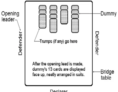
playing against E and W. A standard fifty two pack is used and the cards in each suit rank from the highest to the lowest as Ace (A), King (K), Queen (Q), Jack (J ), 10, 9, 8, 7, 6, 5, 4, 3, 2. The dealer deals out all the cards one at a time so that each player receives 13 of them. The team who made the final bid will at the moment try to make the contract. The first player of this group who mentioned the value of the contract becomes the declarer. The declarer’s partner is well-known as the dummy shown in Fig. 1.
Fig. 1 Bridge playing table
bidding phase when the opponents try to prevent from doing it. In bridge, special focus in game representation is on the fact that players cooperate in pairs, thus sharing potentials of their hands [14].
To estimate the number of tricks to be taken by one pair of bridge players in DDBP, an attempt is made to solve the problem in which the solver is presented with all four hands and is asked to determine the course of play that will achieve or defeat at a particular contract. The partners of the declarer, whose cards are placed face up on the table and may be played by declarer. The dummy has few rights and may not participate in choices concerning the play of the hand and estimating hands strength is a decisive aspect of the bidding phase of the game of bridge, since the contract bridge is a game with incomplete information. This incompleteness of information might allow for many variants of a deal in cards distribution and the player should take into account all these variants and speedily approximate the predictable number of tricks to be taken in each case [15].
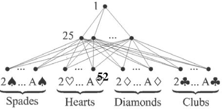
The fifty two input card representation deals were implemented in this architecture. The card values were determined in rank card (2, 3, K, A) and suit card (♠ (S), ♥ (H), ♦ (D), ♣(C)). The rank card was transformed using a uniform linear transformation to the range from 0.10 to 0.90. The Smallest card value is 2(0.10) and highest card value is A (0.90).
ISSN 2348 – 7968
Fig. 2 Neural network architecture with 52 input neurons
Layers were fully connected, i.e., in the 52 − 25 − 1 network all 52 input neurons where connected to all 32 hidden ones, and all hidden neurons were connected to a single output neuron.
2.2. The Bidding and Playing Phases
The bidding phase is a conversation between two cooperating team members against an opposing partnership which aims to decide who will be the declarer. Each partnership uses an established bidding system to exchange information and interpret the partner's bidding sequence as each player has knowledge of his own hand and any previous bids only. A very interesting aspect of the bidding phase is the cooperation of players in North with South and West with East. In each, player is modeled as an autonomous, active agent that takes part in the message process [16, 17].
The play phase seems to be much less interesting than the bidding phase. The player to the left of the declarer leads to the first trick and may play any card and instantly after this opening lead, the dummy's cards are exposed. The play proceeds
clockwise and each of the other three players in turn must, if found potential, play a card of the same suit that the person in-charge played. A player with no card of the suit may play any card of his selection. A trick consists of four cards, one from each player, declared won by the maximum trump in it, or if no trumps were played by the maximum card of the suit. The winner of a trick leads subsequently with any card as the dummy takes no active role in the play and not permitted to offer any advice or observation. Finally, the scoring depends on the number of tricks taken by the declarer team and the contract [18-20].
2.3 No-Trump & Trump-Suit
A trick contains four cards one contributed by each player and the first player starts by most important card, placing it face up on the table. In a clockwise direction, each player has to track suit, by playing a card of the similar suit as the one led. If a heart is lead, for instance, each player must play a heart if potential. Only if a player doesn’t have a heart he can discard. The maximum card in the suit led wins the trick for the player who played it. This is called playing in no-trump. No-trump is the maximum ranking denomination in the bidding, in which the play earnings with no-trump suit. No-trump contracts seem to be potentially simpler than suit ones, because it is not possible to ruff a card of a high rank with a trump card. Though it simplifies the rules, it doesn’t simplify the strategy as there is no guarantee that a card will take a trick,
even Aces are useless in tricks of other suits in no-trump contracts. The success of a contract often lies in the hand making the opening lead. Hence even knowing the location of all cards may sometimes be not sufficient to indicate cards that will take tricks [21]. A card that belongs to the suit has been chosen to have the highest value in a particular game, since a trump can be any of the cards belonging to any one of the players in the pair. The rule of the game still necessitates that if a player can track suit, the player must do so, otherwise a player can no longer go behind suit, however, a trump can be played, and the trump is higher and more influential than any card in the suit led [22].
2.4 Work Point Count System
The Work Point Count System (WPCS) which scores 4 points for Ace, 3 points for King, 2 points for Queen and 1point for a Jack is followed in which no points are counted for 10 and below. During the bidding phase of contract bridge, when a team reaches the combined score of 26 points, they should use WPCS for getting final contract and out of thirteen tricks in contract bridge, there is a possibility to make use of eight tricks by using WPCS.
3. The Data Representation of GIB
library
The data used in this game of DDBP was taken from the Ginsberg’s Intelligent Bridge (GIB) Library, which includes 7,00,000 deals and for each of the tricks, it provides the number of tricks to be taken by N S pair for each combination of the trump suit and the hand which makes the opening lead. There are 20 numbers of each deal i.e. 5 trump suits by 4 sides as No-trumps, spades, Hearts, Diamonds and Clubs.
4. Artificial Neural Networks
ISSN 2348 – 7968 rewards over its counterpart, as it learns at a faster
rate, the network determines its own dimension and topology, it retains the structures it had built, still if the preparation set changes, and it requires no back-propagation of error signals through the associations of the network. During the learning progression, new neurons are added to the network one by one Fig.3 and each one of them is placed into a new hidden layer and connected to all the preceding input and hidden neurons. Once a neuron is finally further to the network and activated, its input connections become frozen and do not change anymore.
Fig. 3 Cascade-Correlation Neural Network (CCNN)
The neuron to be added to the existing network can be made in the following two steps: (i) The candidate neuron is connected to all the input and hidden neurons by trainable input connections, but its output is not connected to the network. Then the weights of the candidate neuron can be trained while all the other weights in the network are
frozen. (ii) The candidate is connected to the output neurons and then all the output connections are trained. The whole process is repeated until the desired network accuracy is obtained. The equation (1) correlation parameter ‘S’ defined as below is to be maximized.
𝑆=� ���𝑉𝑝− 𝑉���𝐸𝑝𝑜− 𝐸����𝑜
𝑃
𝑝=1
�
𝑂
0=1
(1)
The equation (2) where O is the number of network outputs, P is the number of training patterns, VRpR is output on the new hidden neuron and ERpoR is the error on the network output. The weight adjustment for the new neuron can be found by gradient descent rule as
∆𝑤𝑖=� � 𝜎𝑜
𝑃
𝑝=1 𝑂
0=1
�𝐸𝑝𝑜− 𝐸����𝑓𝑜 𝑝ˈ 𝑥𝑖𝑝 (2)
The output neurons are trained using the generalized delta learning rule for faster convergence in Back -Propagation algorithm. Each hidden neuron is trained just once and then its weights are frozen. The network learning building process is completed when satisfied results are obtained. The cascade-correlation architecture needs only a forward sweep to compute the network output and then this information can be used to train the candidate neurons.
5. Back-Propagation (BP) Training
Algorithm
Input n
Input 1
Bias 1 Hidden
2 Hidden
The cascade correlation neural network is a widely used type of network architecture, Instead of just adjusting the weights in a network of fixed topology, with supervised learning. This network consists of an input layer, a hidden layer, an output layer and two levels of adaptive connections [24]. It is also fully interconnected, i.e. each neuron is connected to all the neurons in the next level. The overall idea behind back propagation is to make large change to a particular weight, ‘w’ the change leads to a large reduction in the errors observed at the output nodes. The equation (3) let ‘y’ be a smooth function of several variables xRiR, we want to know how to make incremental changes to initial values of each xRiR, so as to increase the value of y as fast as possible. The change to each initial xRiR value should be in proportion to the partial derivative of y with respect to that particular xRiR. The equation (4) Suppose that ‘y’ is a function of a several intermediate variables xRi Rand that eachR RxRiR is a function of one variable ‘z’. Also we want to know the derivative of ‘y’ with respect to ‘z’, using the chain rule.
∆𝑥𝑖∞𝜕𝑥𝜕𝑦
𝑖 (3)
𝑑𝑦
𝑑𝑧=�
𝜕𝑦
𝜕𝑥𝑖
𝑖
𝑑𝑥𝑖
𝑑𝑧 =�
𝑑𝑥𝑖
𝑑𝑧
𝑖
𝜕𝑦
𝜕𝑥𝑖 (4)
The standard way of measuring performance is to pick a particular sample input and then sum up the squared error at each of the outputs. We sum over all sample inputs and add a minus sign for an
overall measurement of performance that peaks at o.
𝑃=− � ��(𝑑𝑠𝑧
𝑧
−𝑜𝑠𝑧)2�
𝑠
(5)
Where ‘P’ is the measured performance, S is an index that ranges over all sample inputs, Z is an index that ranges overall output nodes, dRsz Ris the desired output for sample input 's' at the zP
th
P
node, oRsz Ris the actual output for sample input 's' at the zP
th
P
node. The performance measure P is a function of the weights. We can deploy the idea of gradient ascent if we can calculate the partial derivative of performance with respect to each digit. With these partial derivatives in hand, we can climb the performance hill most rapidly by altering all weights in proportion to the corresponding partial derivative. The performance is given as a sum over all sample inputs. We can compute the partial derivative of performance with respect to a particular weight by adding up the partial derivative of performance for each sample input considered separately. The equation (6) each weight will be adjusted by summing the adjustments derived from each sample input. Consider the partial derivative
𝜕𝑃
𝜕𝑤𝑖→𝑗 (6)
where the weight 𝑤𝑖→𝑗 is a weight connecting iP
th
P
layer of nodes to jP
th
P
ISSN 2348 – 7968 intermediate variable oRjR, the output of the jP
th
P
node and using the chain rule, it is express as
𝜕𝑃
𝜕𝑤𝑖→𝑗=
𝜕𝑃
𝜕𝑜𝑗
𝜕𝑜𝑗
𝜕𝑤𝑖→𝑗=
𝜕𝑜𝑗
𝜕𝑤𝑖→𝑗
𝜕𝑃
𝜕𝑜𝑗 (7)
Determine oRj R by adding up all the inputs to node
'j' and passing the results through a function.
𝑜𝑗=𝑓 ��0𝑖𝑤𝑖→𝑗
𝑖
� (8)
Hence,
where 𝑓 is a threshold function. Let
𝜎𝑗= �0𝑖𝑤𝑖→𝑗
𝑖
We can apply the chain rule again.
𝜕𝑜𝑗
𝜕𝑤𝑖→𝑗=
𝑑𝑓(𝜎𝑗)
𝑑𝜎𝑗
𝜕𝜎𝑗
𝜕𝑤𝑖→𝑗 (9)
𝜕𝑃
𝜕𝑜𝑗
𝑑𝑓(𝜎𝑗)
𝑑𝜎𝑗 𝑜𝑖
𝜕𝑃
𝜕𝑜𝑘 (10)
𝜕𝑃
𝜕𝑤𝑖→𝑗=𝑜𝑖
𝑑𝑓(𝜎𝑗)
𝑑𝜎𝑗
𝜕𝑃
𝜕𝑜𝑗 (11)
Substituting Equation (8) in Equation (5), we have
𝜕𝑃
𝜕𝑜𝑗=𝜕𝑤𝑖→𝑗
𝑑𝑓(𝜎𝑘)
𝑑𝜎𝑘
𝜕𝑃
𝜕𝑜𝑘 (12)
𝜕𝑃
𝜕𝑤𝑖→𝑗=𝑜𝑖
𝑑𝑓(𝜎𝑗)
𝑑𝜎𝑗 𝑤𝑗→𝑘
𝑑𝑓(𝜎𝑘)
𝑑𝜎𝑘
𝜕𝑃
𝜕𝑜𝑘 (13)
Thus, the two important consequences of the above equations are, 1) The partial derivative of
performance with respect to a weight depends on the partial derivative of performance with respect to the following output. 2) The partial derivative of performance with respect to one output depends on the partial derivative of performance with respect to the outputs in the next layer. The system error will be reduced if the error for each training pattern is reduced. The equation (14) and (15), Thus, at step’s+1' of the training process, the weight adjustment should be proportional to the derivative of the error measure computed on iteration’s’. This can be written as
∆𝑤(𝑠+ 1) =−𝜕𝑤𝑛𝜕𝑃(𝑠) (14)
6. The Resilient Back-Propagation (RBP)
Algorithm
The algorithm RBP is a local adaptive learning scheme, performing supervised batch learning in cascade-correlation neural networks. The basic principle of RBP is to eliminate the harmful influence of the size of the partial derivative on the weight step. As a consequence, only the sign of the derivative is considered to indicate the direction of the weight update.
The algorithm acts on each weight separately. The equation (16) for each weight, if there was a sign change of the partial derivative of the total error function compared to the last iteration, the update value for that weight is multiplied by a factor η−, where 0 <η− < 1. If the last iteration produces the same sign, the update value is multiplied by a factor of η +, where η+ > 1. The update values are calculated for each weight in the above manner, and finally each weight is changed by its own update value, in the opposite direction of that weight's partial derivative. This is to minimize the total error function. η+ is empirically set to 1.2 and η− to 0.5.
To elaborate the above description mathematically we can start by introducing for each weight 𝑤𝑖𝑗 its
individual update value ∆𝑖𝑗 (t), which exclusively determines the magnitude of the weight-update. This update value can be expressed mathematically according to the learning rule for each case based on the observed behavior of the partial derivative during two successive weight-steps by the following formula:
∆𝑖𝑗(𝑡)
=
⎩ ⎪ ⎨ ⎪
⎧𝜂+.∆
𝑖𝑗(𝑡 −1), 𝑖𝑓 𝜕𝑤𝜕𝐸 𝑖𝑗(𝑡).
𝜕𝐸
𝜕𝑤𝑖𝑗(𝑡 −1) > 0
𝜂−.∆
𝑖𝑗(𝑡 −1), 𝑖𝑓 𝜕𝑤𝜕𝐸 𝑖𝑗(𝑡).
𝜕𝐸
𝜕𝑤𝑖𝑗(𝑡 −1) < 0
∆𝑖𝑗(𝑡 −1), 𝑒𝑙𝑠𝑒
(16)
Where 0<𝜂−<1<𝜂+.
ISSN 2348 – 7968
∆𝑤𝑖𝑗(𝑡)
=
⎩ ⎪ ⎨ ⎪
⎧ −∆𝑖𝑗(𝑡), 𝑖𝑓 𝜕𝑤𝜕𝐸
𝑖𝑗(𝑡) > 0
∆𝑖𝑗(𝑡), 𝑖𝑓 𝜕𝑤𝜕𝐸
𝑖𝑗(𝑡) < 0 (17)
0, 𝑒𝑙𝑠𝑒
𝑤𝑖𝑗(𝑡+ 1) =𝑤𝑖𝑗(𝑡) +∆𝑤𝑖𝑗(𝑡) (18)
However, there is one exception. The equation (19) if the partial derivative changes sign that is the previous step was too large and the minimum was missed, the previous weight-update is reverted
∆𝑤𝑖𝑗(𝑡) =−𝑤𝑖𝑗(𝑡 −1),
𝑖𝑓𝜕𝑤𝜕𝐸
𝑖𝑗(𝑡).
𝜕𝐸
𝜕𝑤𝑖𝑗(𝑡 −1) < 0 (19)
Due to that ‘backtracking’ weight-step, the derivative is assumed to change its sign once again in the following step. In order to avoid a double penalty of the update-value, there should be no adaptation of the update-value in the succeeding step. In practice this can be done by setting
𝜕𝐸
𝜕𝑤𝑖𝑗(𝑡 −1) = 0 in the ∆𝑖𝑗 update-rule above.
The equation (20) partial derivative of the total error is given by the following formula:
𝜕𝐸
𝜕𝑤𝑖𝑗(𝑡) =
1 2�
𝜕𝐸𝑝
𝜕𝑤𝑖𝑗
𝑝
𝑝=1
(𝑡) (20)
Hence, the partial derivatives of the errors must be accumulated for all training patterns Fig.4. This indicates that the weights are updated only after the
presentation of all of the training patterns [25]. It is noticed that resilient back-propagation is much faster than the standard steepest descent algorithm.
6.1. RBP Algorithm Architecture
The minimum (maximum) operator is supposed to deliver the minimum (maximum) of two numbers; the sign operator returns +1, if the argument is positive,-1, if the argument is negative
and 0 otherwise. Repeat Compute Gradient 𝜕𝐸
𝜕𝑤(𝑡)
For all weights and biases {
if �𝜕𝑤𝜕𝐸
𝑖𝑗(𝑡 −1)∗ 𝜕𝐸
𝜕𝑤𝑖𝑗(𝑡) > 0� then {
∆𝑖𝑗(𝑡) = minimum (∆𝑖𝑗(𝑡 −1)∗ 𝜂+,∆max )
∆𝑤𝑖𝑗(𝑡) =−sign �𝜕𝑤𝜕𝐸
𝑖𝑗(𝑡)� ∗ ∆𝑖𝑗(𝑡)
𝑤𝑖𝑗(𝑡+ 1) =𝑤𝑖𝑗(𝑡) +∆𝑤𝑖𝑗(𝑡) 𝜕𝐸
𝜕𝑤𝑖𝑗(𝑡 −1) = 𝜕𝐸 𝜕𝑤𝑖𝑗(𝑡)
} else if � 𝜕𝐸
𝜕𝑤𝑖𝑗(𝑡 −1)∗ 𝜕𝐸
𝜕𝑤𝑖𝑗(𝑡) < 0� then {
∆𝑖𝑗(𝑡) = maximum (∆𝑖𝑗(𝑡 −1)∗
𝜂−,∆
mix ) 𝜕𝐸
𝜕𝑤𝑖𝑗(𝑡 −1) = 0
}
else if � 𝜕𝐸
𝜕𝑤𝑖𝑗(𝑡 −1)∗ 𝜕𝐸
𝜕𝑤𝑖𝑗(𝑡) = 0� then {
∆𝑤𝑖𝑗(𝑡) =−sign �𝜕𝑤𝜕𝐸𝑖𝑗(𝑡)� ∗ ∆𝑖𝑗(𝑡)
𝜕𝐸
𝜕𝑤𝑖𝑗(𝑡 −1) = 𝜕𝐸 𝜕𝑤𝑖𝑗(𝑡) 𝜕𝐸
𝜕𝑤𝑖𝑗(𝑡 −1) = 𝜕𝐸 𝜕𝑤𝑖𝑗(𝑡)
Fig. 4 The Resilient Back-Propagation algorithm for learning architecture in CCNN network
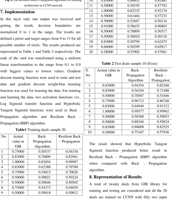
7. Implementation
In this layer only one output was received and getting the result, decision boundaries are normalized 0 to 1 in the range. The results are defined a priori and target ranges from 0 to 13 for all possible number of tricks. The results produced are represented in Table 1 and Table 2 respectively. The rank of the card was transformed using a uniform linear transformation to the range from 0.1 to 0.9 with biggest values to lowest values. Gradient descent training function were used to train and test data and gradient descent weight/bias learning function was used for learning the data. For training and learning the data, two activation functions viz., Log Sigmoid transfer function and Hyperbolic Tangent Sigmoid functions were used in Back - Propagation algorithm and Resilient Back - Propagation (RBP) algorithm.
Table1 Training deals sample 20 S. No Actual
value in GIB
Back- Propagation
Algorithm
Resilient Back – Propagation
1 0.75000 0.50537 0.56336
2 0.83000 0.76809 0.82961
3 1.00000 0.83654 0.99987
4 0.83000 0.62388 0.70788
5 0.75000 0.54815 0.70020
6 0.50000 0.50021 0.50224
7 0.58000 0.50046 0.50565
8 0.75000 0.54373 0.94029
9 0.50000 0.50018 0.50012
10 0.83000 0.84651 0.82685
11 0.58000 0.50195 0.57703
12 1.00000 0.83235 0.92176
13 0.58000 0.61464 0.57233
14 0.50000 0.52667 0.50134
15 0.91000 0.58635 0.90803
16 0.50000 0.78009 0.50317
17 0.50000 0.50010 0.50110
18 0.83000 0.50799 0.62475
19 0.66000 0.50299 0.65817
20 0.58000 0.53902 0.57061
Table 2 Test deals sample 10 (Even) S.
No
Actual value in GIB
Back- Propagation
Algorithm
Resilient Back – Propagation
1 0.83000 0.94354 0.82368
2 0.83000 0.56256 0.71488
3 0.50000 0.70507 0.51046
4 0.75000 0.96712 0.86768
5 0.83000 0.64946 0.91212
6 1.00000 0.99577 0.99962
7 0.50000 0.56368 0.50053
8 0.50000 0.88346 0.59824
9 0.83000 0.88008 0.82525
10 0.58000 0.75167 0.57936
The result showed that Hyperbolic Tangent Sigmoid function produced better result in Resilient Back - Propagation (RBP) algorithm when compared with Back - Propagation algorithm.
8. Representation of Results
ISSN 2348 – 7968 neurons, twenty five hidden neurons and only one
output neuron (52-25-1). The Back Propagation Algorithm and Resilient –Back Propagation Algorithm were used for training and testing through MATLAB 2008a. The results are represented in Fig.5, Fig.6 and Fig.7.
Fig.5 Back Propagation Training deals sampling 1000 epochs
Fig.6 Resilient –Back Propagation Training deals sampling 1000 epochs
Fig.7 Resilient –Back Propagation Testing deals sampling 1000 epochs
The results revealed that, the data trained and tested through Resilient Back - Propagation (RBP) algorithm produced better result in both functions and the time taken for training and testing the data were relatively minimum which also converged to the error steadily during the whole process.
9. Conclusion and Future Works
In Cascade-Correlation neural network, during training process new hidden nodes are added to the network one by one. For each new hidden node, the correlation magnitude between the new node output and the residual error signal is maximized. During the time when the node is being added to the network, the input weights of hidden nodes are frozen, and only the output connections are trained repeatedly. The Work Point Count System used in Resilient –Back Propagation Algorithm which produced better results and used to bid a final contract is a good information system and it provides some new ideas to the bridge players and helpful for beginners and semi professional players in improving their bridge skills. Back – Propagation Algorithm and Resilient – Back propagation algorithms were used in Cascade-Correlation neural network. While comparing these two algorithms, Resilient – Back propagation algorithm produce better result which minimize the mean squared error of the output. The best tested algorithms were capable of discovering
0.00000 0.20000 0.40000 0.60000 0.80000 1.00000 1.20000
1 4 7 10 13 16 19
ERRO
R
NO OF EPOCHS
Back Propagation Resilient –Back Propagation
0.00000 0.20000 0.40000 0.60000 0.80000 1.00000 1.20000
1 4 7 10 13 16 19
ERRO
R
NO OF EPOCHS
Back Propagation Resilient –Back Propagation
0.00000 0.20000 0.40000 0.60000 0.80000 1.00000 1.20000
1 3 5 7 9
ERRO
R
NO OF EPOCHS
acquaintance concerning the game based exclusively on sample training and testing deals. Furthermore we would enlarge the new architecture and algorithm to solve DDBP more efficiently and effectively.
References
[1] Mandziuk,J.(2010). Knowledge-free and Learning – Based methods in Intelligent Game Playing. Springer.
[2] Mandziuk,J.,Mossakowski,K.(2009). Neural Networks compete with expert human players in solving the double dummy bridge problem. In Proceedings of the Conference on Computational Intelligence and games, 5, pp. 117-124.
[3] Dharmalingam,M., Amalraj,R.(2013). Artificial Neural Network Architecture for Solving the Double Dummy Bridge Problem in Contract Bridge, International Journal of Advanced Research in Computer and Communication Engineering, vol. 2, issue.12, pp. 4683-4691.
[4] Dharmalingam,M., Amalraj,R.(2014). Back-Propagation Neural Network Architecture for Solving the Double Dummy Bridge Problem in Contract Bridge, IEEE International Conference on Intelligent Computing Applications, pp. 454-461. [5] Mossakowski,K., Mandziuk,J.(2004). Artificial
Neural Networks for solving double dummy bridge problems. In Lecture Notes in Artificial Intelligence, LNAI: vol, 3070. Artificial
Intelligence and Soft Computing ICAISC, pp.915-921.
[6] Sarkar,M., Yegnanarayana,B., Khemani,D.(1995). Application of neural network in contract bridge bidding. In Proceeding of National Conference on Neural Networks and Fuzzy Systems, Madres, pp.144-151.
[7] Dharmalingam,M., Amalraj,R.(2013).Neural Network Architectures for Solving the Double Dummy Bridge Problem in Contract Bridge. In Proceeding of the PSG-ACM National Conference on Intelligent Computing.1, pp.31-37. [8] Frank,I., Basin,D.A.(1999). Optimal play against
best Defence: Complexity and Heuristics. In Lecture Notes in Computer Science, vol, 1558, Germany, pp. 50-73.
[9] Smith,S.J.J., Nau,D.S.(1994). An Analysis of Forward Pruning. In Proceeding of the National Conference on Artifitical Intelligence, pp.1386-1391.
[10]Smith,S.J.J., Nau,D.S., Throop,T.A.(1998). Success in Spades: Using AI Planning Techniques to Win the World Championship of Computer Bridge. In Proceeding of the National Conference on Artificial Intelligence, pp.1079-1086.
[11]Francis,H.,Truscott,A., Francis,D.(1940). The Official Encyclopedia of Bridge, American Contract Bridge League.(5th) Edition.
ISSN 2348 – 7968 [13]Mandziuk,J.(2007). Computational Intelligence in
Mind Games, Springer.
[14]Mossakowski,K., Mandziuk,J.(2009). Learning without human expertise: A case study of Double Dummy Bridge Problem. IEEE Transactions on Neural Networks, 20(2), pp. 278-299.
[15]Dharmalingam,M., Amalraj,R.(2013). Supervised Learning in Imperfect Information Game. International Journal of Advanced Research in Computer Science,4(2), pp. 195-200. [16]Yegnanarayana,B., Khemani,D., SarkarM.(1996). Neural Network for contract bridge bidding. 21(3), pp. 395-413.
[17]Amit,A.,Markovitch,S.(2006). Learning to bid in bridge. Machine Learning, 63(3), pp. 287-327. [18]Smith,S.JJ., Nau,D.S., Throop,T.A.(1998).
Computer Bridge - A Big Win for AI planning. Artificial Intelligence Magazine, 19(2), pp. 93-106.
[19]Frank,I., Basin,D.A.(2001). A Theoretical and Empirical Investigation of Search in Imperfect Information Game. Theoretical Computer Science, 252(1), pp 217-256.
[20]Ando,T., Sekiya,Y., Uehara,T.(2010). Partnership bidding for Computer Bridge. Systems and Computers in Japan, 31(2), pp.72-82.
[21]Jamroga,W.(1999). Modeling Artificial Intelligence on a case of bridge card play bidding. In Proceedings of International
Workshop on Intelligent Information System, pp. 276-277.
[22]Mandziuk,J.(2008). Some thoughts on using Computational Intelligence methods in classical mind board games. In Proceedings of the International Joint Conference on Neural Networks, pp. 4001-4007.
[23]Fahlman,S.E, Lebiere,V.(1990). The cascade-correlation learning architecture. Advances in Neural Information Processing, pp. 524-532.
[24]Rumelhart,D.E., Hinton,G.E.,
Williams,R.J.(1986). Learning internal representations by error backpropagation, Parallel Distributed Processing: Ex-plorations in the Microstructure of Cognition, vol. 1, pp. 533-536.
Authors Biography
Dr. M Dharmalingam received his Under-Graduate, Post-Graduate and Master of Philosophy degrees from Bharathiar University, Coimbatore in the years 2000, 2004 and 2008 respectively. Currently he is working as an Assistant Professor in Computer Science, Nandha Arts and Science College, Erode and also pursuing part time PhD degree in Computer Science at Sri Vasavi College, Bharathiar University, Tamil Nadu, India. He has published several research papers in reputed National and International journals and the broad field of his research interest is Soft Computing.
Dr. R Amalraj is working as an Associate Professor in Computer Science, Sri Vasavi College, Erode, Tamil Nadu, India. He has obtained his PhD in Computer Science from PSG College of Technology, affiliated to Bharathiar University, Coimbatore in 2003. He is a Life Member of Computer Society of India. He has been a Principal