University of South Carolina
Scholar Commons
Theses and Dissertations
2018
The Visual Ecology of Speyeria mormonia
Natalie Sanchez Gonzalez
University of South Carolina - Columbia
Follow this and additional works at:https://scholarcommons.sc.edu/etd
Part of theBiological Engineering Commons
This Open Access Dissertation is brought to you by Scholar Commons. It has been accepted for inclusion in Theses and Dissertations by an authorized administrator of Scholar Commons. For more information, please [email protected].
Recommended Citation
The Visual Ecology of
Speyeria mormonia
by
Natalie Sanchez Gonzalez
Bachelor of Arts
The University of Pennsylvania, 2016
Submitted in Partial Fulfillment of the Requirements
For the Degree of Master of Science in
Biological Sciences
College of Arts and Sciences
University of South Carolina
2018
Accepted by:
Daniel I. Speiser, Director of Thesis
Carol Boggs, Reader
Jeff Dudycha, Reader
ii
iii
DEDICATION
I would like to dedicate this thesis to my parents, grandparents, and my friends
who were my emotional support during the toughest moments of this entire process. I
love you all and I couldn’t have finished this without your prayers, phone calls, and
iv
ACKNOWLEDGEMENTS
I acknowledge Dr. Soumitra Goushrouy, Dr. Shannon Davis, and the faculty at
the IRF facility of the medical school who helped me troubleshoot the protocols for the
microscopic imaging of butterfly eyes. I also acknowledge Dr. Nate Morehouse for
sharing his template with me which facilitated the completion of the computational model
for the spectral sensitivity of S. mormonia. I acknowledge Dr. Carol Boggs for her
research guidance and her research assistants, especially Lydia Fisher, Emma Wagner,
Hannah Whitton, Skylar McDaniel, and Malia Olson for helping me collect and care for
butterflies out in the field and at the Rocky Mountain Biological Laboratory. I
acknowledge Rebecca Lucia for helping me care for the butterflies and take photographs
of them. I acknowledge Rachel Steward for providing a variety of helpful resources for
this research project. Finally, I acknowledge Luke Havens, our research specialist, who
v ABSTRACT
Variations in environmental factors such as temperature, precipitation, and day
length during larval development are known to affect morphological traits in butterflies
related to their visual ecology, including eye size and wing color. These vision-related
traits are important for the ability of diurnal butterfly species to detect mates, especially
at long distances. Thus, changes in environmental conditions may result in phenotypic
modifications to butterflies which may alter their visual ecology and subsequently, their
reproductive fitness. To study the interaction of phenotypic plasticity and visual ecology
in the Mormon Fritillary, Speyeria mormonia, I set up a natural-laboratory experiment at
the Rocky Mountain Biological Laboratory (RMBL) and collected butterflies from 5
different sites across an elevational gradient, spanning approximately 610 meters during
two field seasons. I considered elevation to be a proxy for several shifting microclimate
features, including temperature and precipitation. My first goal was to determine whether
there was a relationship between elevation and natural variations in the dorsal wing
chromaticity, eye surface area, or wing length (a proxy for body size) of male and female
adult-stage S. mormonia from the study populations. In the case that I did find natural
variations in wing chromaticity, my second goal was to use computational models to
evaluate whether S. mormonia can discriminate between the different “oranges”
(quantified using chromaticity values) displayed on the wings of their conspecifics.
Across elevations, I found that females tended to be larger than males and that males
vi
elevations had longer wings than individuals from higher elevations. Males had greater
and more variable wing wear scores than females, and more perceivable variations in
dorsal forewing and dorsal hindwing chromaticity, the values of which were linked to
wing wear. The results also suggest that S. mormonia may have sex-dependent dynamics
in the investment of nutrient resources. Females had longer wing lengths and more
consistent wing wear scores than males across elevations. Longer wings are useful for
female butterflies to maintain more efficient flight maneuverability while carrying heavy
egg-loads during oviposition. Males, however, had larger eyes and more variable wing
wear scores than females. Males may have larger eyes than females because vision is
more important for mate location by males than it is for oviposition site location or
mate-recognition by females. This may mean that while females are investing in producing
larger bodies to optimize fecundity, males are investing nutritional resources into
optimizing mate-seeking ability (i.e. patrolling) to maximize the number of copulations
they can engage in. Finally, intersexual trends in wing wear scores suggest that there are
different degrees of protandry occurring across the elevational gradient, likely because of
vii
TABLE OF CONTENTS
Dedication ... iii
Acknowledgements ... iv
Abstract ...v
List of Tables ... viii
List of Figures ... ix
List of Symbols ... xi
List of Abbreviations ... xii
Chapter 1: Introduction ...1
Chapter 2: Materials and Methods ...6
Chapter 3: Results ...24
Chapter 4: Discussion ...44
viii
LIST OF TABLES
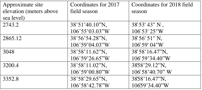
Table 2.1: List of latitude and longitude coordinates corresponding to the field collection sites visited in 2017 and 2018 ...7
Table 2.2: Routine H&E Staining Protocol and chemical wash schedule for the Leica Autostainer XL...11
Table 3.1: Color discriminability values corresponding to comparisons between the average reflectance spectra of male and female dorsal hindwings from 2017 and 2018 ..41
ix
LIST OF FIGURES
Figure 2.1 Diagram of linear measurements obtained from S. mormonia used to estimate
eye surface area ... 10
Figure 2.2 Image of a Hematoxylin and Eosin stained cryosection ...12
Figure 2.3 Image of a corneal spread from S. mormonia ...13
Figure 2.4 Image of S. mormonia wing regions from which reflectance spectra were measured ...15
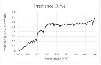
Figure 2.5 Irradiance curves used in computational models...22
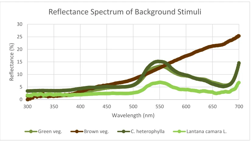
Figure 2.6 Reflectance spectra of background stimuli used in computational models ...23
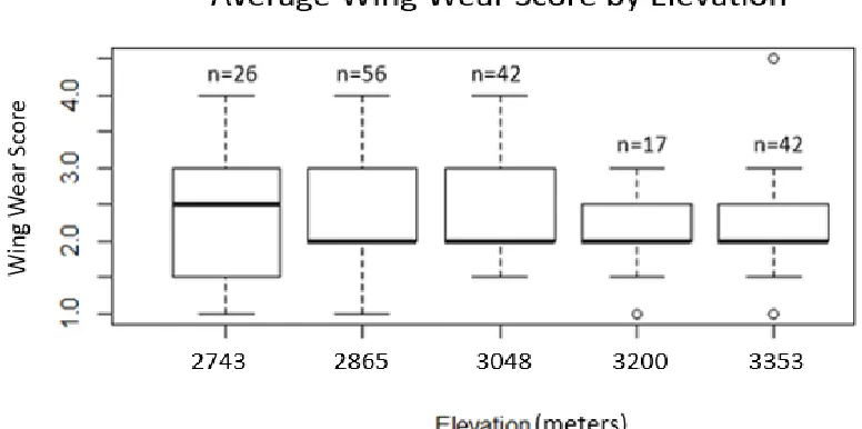
Figure 3.1 Wing wear score by elevation ...25
Figure 3.2 Wing wear score by sex ...25
Figure 3.3 The effect of the interaction between elevation and sex on average wing wear scores ...26
Figure 3.4 Average wing length by sex ...27
Figure 3.5 The effect of the interaction between elevation and sex on average wing length ...28
Figure 3.6 Average wing length by elevation ...29
Figure 3.7 Wing length by field collection year ...29
Figure 3.8 Wing length by wing wear score ...30
Figure 3.9 Average wing lengths of males and females by year of collection ...30
Figure 3.10 Average estimated eye surface area by sex ...31
x
Figure 3.12 Average estimated eye surface area of male and female S. mormonia by
elevation, 2017 ...32
Figure 3.13 Average facet area per eye region for males and females ...33
Figure 3.14 Average rhabdom length per eye region for males and females ...34
Figure 3.15 Eye surface area has a slight negative correlation to wing length in butterflies collected in 2017 ...35
Figure 3.16 Dorsal forewing chromaticity values by wing wear score ...35
Figure 3.17 Dorsal forewing chromaticity by collection year ...36
Figure 3.18 Dorsal forewing chromaticity by sex ...36
Figure 3.19 Dorsal hindwing chromaticity by wing wear score ...37
Figure 3.20 Dorsal hindwing chromaticity by year ...37
Figure 3.21 Average magnitude of response (MoR) curve ...39
Figure 3.22 MoR and visual pigment absorbance curves ...40
Figure 3.23 Color discriminability values (∆St) corresponding to dorsal hindwing and forewing stimulus pairs from 2017 field-caught butterflies (𝜔=0.01)...42
xi
LIST OF SYMBOLS
Ai Absorbance of photoreceptor i
ei Estimate of noise originating from photoreceptor i
I (λ) Irradiance in units of photon flux (𝜇mol/m-2s-1nm-1) at a given wavelength
qi Photon catch of photoreceptor i
RB(λ) Reflectance of the background stimulus at a given wavelength
R(λ) Reflectance of a color stimulus at a given wavelength
xii
LIST OF ABBREVIATIONS
DF chroma ... Dorsal forewing chromaticity
DH chroma ...Dorsal hindwing chromaticity
EESA... Estimated Eye Surface Area
RL ... Rhabdom length
RMBL ... Rocky Mountain Biological Laboratory
∆St ... Color discriminability
WL ... Wing length
1
CHAPTER1
INTRODUCTION
Visual ecology is a field of study which investigates how organisms acquire
visual information and how their visual systems change or become specialized in
response to selection pressures experienced in their natural environments (Cronin 2014).
Butterflies are a classic model in visual ecology because they tend to have excellent color
vision and colorful wings. Butterflies have apposition compound eyes, which are
composed of thousands of subunits called ommatidia. Each ommatidium is covered by a
facet lens and samples light from a small area from the surrounding environment. The
integration of information from multiple ommatidia produces a “pixelated” image of the
world, where each ommatidium is equivalent to one pixel. Wider facets not only increase
sensitivity, but also improve visual resolution by decreasing the blurring effects of
diffraction (Land and Nilsson 2012). Male butterflies typically have larger eyes than
females do, presumably to detect potential mates more efficiently. Males even have
exclusive areas of greater relative visual acuity and sensitivity along the frontal region of
their eyes, called acute or “love” zones (Rutowski 2000). These “love” zones are
characterized by larger facets, longer rhabdoms, and smaller interommatidial angles.
Butterflies also have notoriously colorful wings, the hues of which are produced by the
interaction of light with pigments on the wing scales (Stavenga et al. 2014). These wing
2
courtship. For the most part in butterflies, females tend to be the choosier sex and males
tend to be the more brightly colored sex (Robertson et al. 2005; Kirkpatrick 1982)
The visual sensory modality is known to be important for mate detection in
diurnal butterflies, especially when they need to detect mates from long distances
(Hidaka 2010; Li et al. 2017). Given the importance of visual cues to butterflies for
conspecific recognition, changes in their wing color or wing or eye morphology may alter
their visual ecology by enhancing or diminishing the efficiency of their mating signals
(i.e. the wing colors) or the efficiency with which the receiver can perceive such signals
(White et al. 2015). One of the ways that butterfly wing and eye morphology might
change is through phenotypic plasticity, which is defined as modifications of phenotypes
in response to environmental factors which do not come about as a result of genetic
changes. There is evidence of phenotypic plasticity in wing morphologies and eye sizes
driven by environmental conditions in several species of butterfly, including Bicyclus
anynana and Precis coenia. These butterfly species are known to develop seasonal wing
and eye morphologies that are influenced during larval or pupal development periods by
environmental factors such as temperature, daylength, and precipitation patterns (Smith
1993; Van Bergen et al. 2017). The quantity or quality of larval food sources, which are
directly related to the aforementioned environmental factors, can also promote seasonal
variations in morphological aspects of butterfly visual systems, including eye size or
brain size (Merry et al. 2011; Snell-Rood 2014; Montgomery et al. 2016).
In this study, I asked if variations in eye size, body size, or wing color occur along
an elevational gradient due to differences between the microclimates at each site. To
3
Biological Laboratory (RMBL) using a study population of local Speyeria mormonia.
Butterflies were sampled from 5 different elevation sites spanning approximately 610
meters. This species of butterfly is protandrous and belongs to the family Nymphalidae.
Protandrous species are characterized by males that emerge from the pupal stage earlier
than female conspecifics. S. mormonia are typically found along mountainous ranges in
open grasslands containing various species of Compositae, which is their adult food
source, and Viola spp. host plant which is their larval food source. The various
microclimates within the native range of S. mormonia makes it so that their larvae
experience different environments during development based on the location at which
eggs were laid. My first goal was to quantify inter-elevational differences between traits
in S. mormonia that are relevant to their visual ecology, including wing color, eye size,
and wing size. I obtained wing length and eye measurements by using image analysis
software on scaled microscopic images of the butterflies. I used chromaticity, defined as
the linear slope in reflectance between the wavelengths of 500 and 600 nm, as a proxy for
how “orange” the wing colors were. Based on existing scientific literature, I had reason to
believe that the varying microclimates at each elevational site would yield much natural
variation in wing color and eye morphology. The second goal of this study was to
determine whether the S. mormonia of these sample populations can distinguish between
the naturally occurring variations of “orange” color on the wings of conspecifics within
their natural range using output values from a computational model. Results from the
computational model indicate whether differences in wing color effect the efficiency with
4
I expected that males would have larger eyes than females, but that females would
have longer wings (a proxy for body size) than males regardless of the elevation from
which they were collected. These sexual dimorphisms are common in most protandrous
butterfly species (Rutowsi et al. 2000). If wing color, as a product of diet-dependent wing
pigment production, were primarily affected by the availability of larval food resources
(Lindstedt et al. 2010), I expected that low elevation butterflies would be more chromatic,
given that precipitation and temperature both generally tend to have negative
relationships with elevation, but are directly related to plant yield (Laiolo et al. 2013).
However, snow-pack tends to be greatest at higher elevations in this region, which
increases the local soil moisture. Therefore, the host plant abundance may be greatest at
higher elevations, so there is an alternate possibility that butterflies at higher elevations
will be more chromatic instead. I also expected S. mormonia to be able to discriminate
between a wide variety of “orange” colored wings due to the functional importance of
this color as a cue for mating behavior (Carol Boggs, personal communication).
Finally, although the examples I have offered so far involve trait modifications as
outcomes of phenotypic plasticity, any observable variations in morphology between
these S. mormonia populations could be at least partially influenced by local adaptation.
No prior work has been done on the population genetics of the S. mormonia populations
within Gothic County, CO, so I am unsure of the degree of within population variation or
gene flow occurring between the butterfly communities. The average traveling dispersal
distance of S. mormonia is 170 meters (Boggs 1987), but this is subject to change from
year to year and includes non-linear ("zig-zag") displacement. The average linear
5
sites were generally closer to each other than the sites at lower elevations. The
approximate Wrightian neighborhood distance, or geographic space where S. mormonia
are more likely to be directly related to each other (Watt et al. 1977; Wright 1946), is
roughly 875 meters (Dr. Boggs personal communication). Therefore, given the variation
in dispersal distances within S. mormonia populations and the dearth of scientific
literature on the population genetics of S. mormonia from this region, any phenotypic
variations observed between butterflies cannot be linked to phenotypic plasticity with
6
CHAPTER 2
MATERIALS AND METHODS
2.1 STUDY ORGANISMS
2.1.1 Study site and field collection
I collected S. mormonia, with the help of research assistants, from 5 different
elevations near the Rocky Mountain Biological Laboratory in Crested Butte, CO.
Collection took place during two field seasons; the first during mid to late August of
2017 and the second during late July through early August of 2018. The collection sites
were located at 2743, 2865, 3048, 3200, and 3353 meters above sea level (Table 2.1). In
2017, I net-captured butterflies and transported them to the lab. In the lab, I fed butterflies
25% sugar water. I photographed all butterflies on graph paper with subdivisions of
known length which I used for scale, using a Canon Powershot A4000 camera. I
photographed the butterflieswithin 24 hours of their being captured. I then released the
majority of the captured butterflies. Butterflies collected in the 2018 field season were
caught using the same protocol, but none were released. They were fed, stored in small
envelopes, placed in a box, and shipped overnight to the University of South Carolina.
7
chilled incubator under full spectrum light (20” Aqueon modular LED Aquarium light)
and a light:dark cycle of 12h:12h. The temperature schedule was set to 19˚C by day and
17˚C by night. I photographed the butterflies using a Nikon D5000 camera and measured
their wing lengths using electronic calipers. For spectral reflectance measurements, I used
a subset of wings from male and female S. mormonia collected in 2017 and the wings
from all the butterflies collected in 2018.
Table 2.1: List of latitude and longitude coordinates corresponding to the field collection sites visited in 2017 and 2018.
Approximate site elevation (meters above sea level)
Coordinates for 2017 field season
Coordinates for 2018 field season
2743.2 38˚51’40.10”N,
106˚55’03.03”W
38̊ 53' 43" N , 106̊ 53' 25"W
2865.12 38˚56’54.28”N,
106˚59’04.03”W
38̊ 56' 51" N, 106̊ 59' 04"W
3048 38˚58’11.62”N,
106˚59’26.65”W
38̊ 58’16.47”N, 106̊ 59’34.40”W
3200.4 38˚58’11.02”N,
106˚59’00.80”W 38̊58’29.12”N, 106̊ 58’40.70” W
3352.8 38˚58’29.65”N,
106˚58’42.78”W
38̊58’16.47”N, 106̊59’34.40”W
2.1.2 Lab rearing S. mormonia
S. mormonia from RMBL were transferred as first instar larvae to the University
of South Carolina in glass 1.5 mL vials in the fall of 2017. They were held at 2°C for 5
months and brought out of diapause in the spring of 2018. After diapause, larvae were
raised on host plants, Viola soraria, under full spectrum light on a 16h:8h light:dark cycle
and a 27°C:15°C temperature cycle. Pupae were weighed, logged into our butterfly
8
with mesh. Pupae were spritzed with water daily to maintain a rearing environment
humid enough to promote successful wing extension upon eclosion as adults. Upon
eclosion, each butterfly’s emergence date, wing length, and sex were recorded. For 2-4
weeks post-eclosion, adult females were transferred into an incubator with a light:dark
cycle of 16h:8h under full spectrum light and temperatures at 27̊C:15̊C day:night. They
were fed 25% sugar water twice a day. Males were placed in groups of 3-4 into separate
cylindrical plastic containers with moistened paper towels inside to maintain humidity
levels. They were fed 25% sugar water once a day. The eyes of a subset of males and
females from this lab-reared population of butterflies were excised and fixed for
histology within 24 hours after death.
2.2 EYE AND WING MORPHOLOGY
2.2.1 Wing wear scores
Wing wear scores are categorical scores assigned to butterflies estimating the
degree to which their wings have been worn. The score ranges from 1, for freshly
emerged butterflies with moist wings without any wear, to a score of 5, for butterflies
which have very noticeable scale loss and significant wing tearing that goes beyond the
borders (Boggs 1987). A score of 2 is given to adults with dry wings but no wear. Up to
1.5 points, in increments of 0.5, are then added for scale loss (color loss), and an
additional 1.5 points are added, in increments of 0.5 for wing tearing/loss.Wing wear can
be used as a proxy for age. Wing wear scores were assigned to all field-caught butterflies
9
2.2.2 Wing length measurements
Wing length is the linear distance from the basal hinge of the forewing to the tip
of the forewing. I measured the wing lengths of field-caught S. mormonia collected
during the first field season by making linear measurements of wings from photographs
of butterflies lying on graph paper with subdivisions of 0.1 cm, which I used for scale. I
measured the wing lengths of S. mormonia from the second field collection season using
electronic calipers.
2.2.3 Estimated eye surface area
I estimated the surface areas of eyes from S. mormonia by taking linear
measurements of the eye height and 3 different eye radii from scaled images of
S. mormonia heads. I used the subdivisions on the graph paper background for scale, as
explained above. Given that the eye height measurements were consistently less than 2
times the average radius value, I modeled the eyes as oblate spheroids. I plugged the
linear measurements into the formula corresponding to the surface area of an oblate
spheroid to estimate eye surface area (Rutowski 2000).
2.2.4 Hematoxylin and Eosine Staining and imaging of S. mormonia rhabdoms
I obtained average rhabdom lengths by performing light microscopy on images of
cryosections of eyes from lab-reared S. mormonia. Within 24 hours after death, I excised
butterfly heads, cut them in half, and fixed them in 2% glutaraldehyde, 2%
paraformaldehyde in 0.1 M Phosphate-buffered saline (PBS) overnight. After fixation, I
10
10%, 20%, and 30% sucrose in 0.1M PBS, for 1 hour per wash. After this, I placed the
eyes individually into plastic molds, embedded them in OCT gel (Sakura Tissue Tek
Figure 2.1: A diagram depicting the various measurements of radius (ER1-ER3) and eye height (EH) that I obtained from individual S. mormonia, using image analysis software, to estimate eye surface area. Figure reproduced from Rutowski (2000).
Tokyo) and placed them into a -20̊ freezer until the gel became completely opaque. Once
frozen, I used a Leica CM1850 cryostat (Buffalo Grove, IL) to cut the molds into
16-20-micron thick sections. To improve the contrast of the microscope images, I labeled them
with Hematoxylin and Eosine (H&E), which combine to stain nucleic acids violet and
proteins, membranes, and tissues different shades of pink. I put my cryosections through
a chemical treatment schedule, described on table 2.2, on a Leica Autostainer XL (model:
ST5010, Buffalo Grove, IL). After staining, I imaged the cryosections under an Olympus
CX31 light microscope. I took photographs of the microscope images using a Nikon
11
Table 2.2 Routine H&E Staining Protocol and chemical wash schedule for the Leica Autostainer XL.
Treatment Duration/Notes
95% Alcohol 5 min
Water Wash Rinse
Hematoxylin stain 7 minutes
Water wash Rinse
Acid alcohol 1 dip
Water wash Rinse
Ammonia water 30 sec
Water wash Rinse
Eosin (made up fresh) 5 drops, 2 minutes
95% alcohol 3x. 5 minutes/wash
100% alcohol 2 washes, 5 minutes/wash
12
2.2.5 Corneal extractions
I froze the excised heads of 49 S. mormonia (nf=31, nm=18) in a -20̊ freezer to
prepare them for corneal extractions. I adapted this technique from Ziemba and Rutowski
(2000) to obtain eye surface area and facet area measurements for different regions of the
eyes of S. mormonia.To soften the corneal layer, I removed the eyes from the freezer and
placed them into 10% aqueous NaOH solution for 20 to 25 minutes.
13
I transferred the eyes to a dissecting scope for the removal of the cornea. I marked the
dorsal regions of the eyes with whiteout. This allowed me to determine the orientation of
the different eye regions of interest on the corneal surface. I used fine dissecting scissors
to cut around the perimeter of the eyes and fine forceps to carefully pull the cornea away
from underlying soft structures. I made cuts at the ventral, dorsal, medial, lateral, and
diagonal regions of the extracted corneal layer to spread it flat on the slides. If the cornea
was rigid, I added more 10% NaOH to soften the tissue. Once the cornea was extracted
and flattened, I added 2-3 drops of glycerol to the corneal spreads and placed a cover slip
over them. They were sealed using EM grade clear nail polish. I imaged the slides under
14
a Leica M165FC fluorescent stereo microscope with a DFC295 camera attachment
(Buffalo Grove, IL) at 3.2x and 8x magnification with an ocular micrometer for scale. I
then processed scaled images with ImageJ. To obtain average facet area measurements, I
focused on areas within 9 different quadrants of the corneal surface, corresponding to the
dorsal-medial (quadrant 1), -central (quadrant 2), and -lateral (quadrant 3),
equatorial-medial (quadrant 4), -central (quadrant 5), and -lateral (quadrant 6), and ventral-equatorial-medial
(quadrant 7), -central (quadrant 8), and -lateral (quadrant 9), regions of the eye (Ziemba
and Rutowski 2000). Within each quadrant, I measured the area of the selected region of
space and counted the facets within this region. I calculated average facet area by
dividing the area value by the number of facets counted in units of 𝜇m2/facet.
2.3 SPECTROSCOPY
I took reflectance measurements from wings of 29 field-caught butterflies (15
females, 14 males) collected in 2017 from sites which were 2743, 3048, 3200, and 3353
meters above sea level in elevation. I also took reflectance measurements from a total of
94 wings (56 females and 37 males) of butterflies collected in 2018, from all five of the
elevations sampled. I took measurements from the dorsal forewings and dorsal hindwing
of each butterfly. I used an Ocean Optics Flame spectrometer with a QR400-7-uv-vis
fiber optic cable (Dunedin, FL) and a spectralon, certified reflectance standard by
Labsphere (North Sutton, NH) to get spectral reflectance recordings. I placed samples
onto a spectrally flat, black background with near 0% reflectance. Then, using a probe
holder, I oriented the collection probe at 45̊ below the zenith, and then placed the probe
holder on top of the wing sample. I calculated the chromaticity values from spectral
15
reflectance curve between 500 and 600 nm. The chromaticity value indicates how pure
the specific wavelength of visible light or color is to the viewer. A higher slope value
indicates greater chromaticity and corresponds to a wing which would look more
“orange” to humans. Lower chromaticity values correspond to more “yellow” or “less
saturated orange” looking wings.
16
2.4 COMPUTATIONAL MODELLING OF VISUAL SENSITIVITY
2.4.1 Electroretinography
I assisted Luke Havens in performing electroretinography on 3 male and 3 female
S. mormonia, all of which were lab-reared, aged between 2-4 weeks old (Caves et al.
2016). We began by anesthetizing the butterflies on ice for 15-30 minutes until immobile,
and then excised their protruding appendages (antenna, legs, etc.). We then affixed a
plastic rod onto the dorsal side of the butterfly using hot wax, and then oriented the insect
so that its anterior eye region faced the light source and objective lens. We used Tungsten
microelectrodes, made by electrolytic sharpening. We pushed one electrode into the
retina of the right eye to record electrical responses to light stimuli. We placed a
reference electrode in the left eye of the butterfly and a ground electrode in the head or
abdomen of the insect. The doors of the light-tight Faraday cage, lined with black felt,
were closed. We dark adapted butterflies for 15 minutes before exposing them to light.
The light was produced by a 150 W tungsten-halogen lamp (tungsten-halogen lamp,
Spectral Products, ASBN-W150-PV). Light intensity was controlled by a neutral density
filter wheel (Edmund Optics, model #54-082). We randomly exposed butterflies to
wavelengths of light ranging from 400-700 nm (separated by intervals of 10 nm) using a
monochromator (Monochromator: Spectral Products, CM110). A computer-controlled
shutter (Uniblitz LS3) controlled the duration of light exposure. The different
wavelengths we used as stimuli were presented in random order, each lasting for 1
second, with 9 second time lapses separating the flashes of light throughout the
experimental runs. We ran the same procedure two times for each insect. DC recordings
17
AC/DC amplifier), digitized, and stored in LabView with a custom program developed
by Luke Havens. I accessed and analyzed the ERG data using ADInstruments PowerLab
(8/35). To analyze spectral sensitivity information obtained from the ERG data, I
calculated the magnitude of response (MoR), defined as the absolute value of the
difference between the peak and trough of the voltage response, for each wavelength used
in the light trials. I normalized the MoR values to 1 and averaged them across trials for
each insect. I then pooled the averages from all 3 males and females, averaged them, and
plotted them against wavelength. The wavelengths of maximum absorbance for the short,
medium, and long wavelength sensitive visual pigments most applicable to my models
were 385, 470, and 550 nm, respectively (Yuan et al. 2010). These wavelengths were
plugged into a visual pigment sensitivity template developed by Stavenga et al. (1993) to
get the alpha absorbance curves corresponding to each visual pigment type. I used
Microsoft Excel to plot the alpha absorbance curves corresponding to the three visual
pigments against the MoR curve obtained from ERG data analysis. This allowed us to
determine which wavelengths of maximum sensitivity in the long-wavelength range was
most likely to produce the sensitivity peaks on the MoR curve, by inspection of the
graph. This ultimately gave us an idea of what the spectral sensitivity curve looks like for
S. mormonia.
2.4.2 Computational Model of Color Discriminability
In order to determine whether S. mormonia are able to distinguish between
inter-sexual and inter-elevational variances in wing chromaticity, I used a photoreceptor-noise
limited visual sensitivity model developed by Vorobyev and Osorio (1998). I completed
18
template provided by Dr. Nate Morehouse (personal communication). From this model, I
was able to obtain color discriminability (∆St) output values. A ∆St value is a
quantitative unit of measure corresponding to color discriminability. It indicates how
discriminable the colors of two different stimuli are from each other. A ∆St value that is
greater than 1 indicates that the butterflies can discriminate between the “colors” of two
stimuli based on their individual reflectance spectra; if the ∆St value is less than 1, the
two stimuli are indistinguishable. The greater the value of ∆St, the better they can
discriminate between the two stimuli. Given our dearth of equipment to conduct
epi-microspectrophotometry, I used existing scientific literature about the phylogenetic
relatedness between the short-, medium-, and long- wavelength sensitive rhodopsin
proteins across several butterfly species to have an idea of the absorbance maxima which
are most applicable to the S. mormonia visual system and of the retina-wide relative
abundances of different photoreceptor types. This information was used to determine the
input values for the model. Most butterflies in the family Nymphalidae are trichromatic.
Therefore, I used a template pertaining to the visual system of Hymenoptera, which are
also trichromatic and like nymphalid, possess three major visual opsin types with peak
sensitivities in the UV (300-400 nm), Blue (400-500 nm), and Green (500-600 nm)
wavelength ranges of visible light. A typical ommatidium of a nymphalid contains 9
photoreceptors distributed throughout the distal, proximal, and basal end of the rhabdom.
The blue- and UV-sensitive visual opsins are distributed in the distal R1 and R2
photoreceptors, but the green-wavelength sensitive opsins are in the proximal R3-8
photoreceptors. Long wavelength sensitive opsins have also been identified in the 9th
19
nymphalid butterfly, is 420 micrometers (Briscoe et al. 2003), which is close to the
average rhabdom length I calculated for male S. mormonia, which was 437 𝜇m. The
wavelengths corresponding to the visual pigment sensitivity peaks of S. mormonia’s
closest relatives, including Dryas iulia and Speyeria leto, are 385, 470, and 550 nm
(Yuan et al. 2010). I set the relative abundance of UV-:Blue-:Green- sensitive
photoreceptors to 4.78:1:17.33 in this model, based on the photoreceptor distribution
discovered in Vanessa cardui (Briscoe et al. 2003). This species has the same basic
ommatidia morphology as most other nymphalid butterflies. I plugged these values into
Vorobyev and Osorio’s (1998) receptor noise limited model of spectral sensitivity, to
obtain a measure of color discriminability in units of ∆St (Morehouse and Rutowski
2010). The following formulas were used to calculate the color discriminability between
different pairs of stimuli.
𝑖 = 1,2, … , 𝑛; 𝑞𝑖 is the quantum catch of photorecetor i,
𝑞𝑖 = ln (𝑄𝑖 𝑄𝑖𝐵)
𝑄𝑖 = ∫ 𝑅(𝜆)𝐼(𝜆)𝐴𝑖(𝜆)𝑑𝜆,
𝑄𝑖𝐵 = ∫ 𝑅𝐵(𝜆)𝐼(𝜆)𝐴𝑖(𝜆)𝑑𝜆,
𝑒𝑖 = 𝜔√ 𝑛𝑗
𝑛𝑖
20
(Δ𝑆𝑡)2 =(𝑒12)(Δ𝑞3−Δ𝑞2)2+(𝑒22)(Δ𝑞3−Δ𝑞1)2+(𝑒32)(Δ𝑞1−Δq2)2
(𝑒1𝑒2)2+(𝑒1𝑒3)2+(𝑒2𝑒3)2
Here, qi represents the photon catch value for each photoreceptor given adaptation
to the background stimulus, where λ is the wavelength, R is the reflectance of the
stimulus, RB is the reflectance of the background, I is the irradiance (𝜇mol/m-2s-1nm-1),
and Aiis the absorbance of photoreceptor i (Vorobyev and Osorio 1998). Absorbance
curve corresponding to the three photoreceptor types were obtained by plugging the
wavelengths of maximum sensitivity for each photoreceptor into a formula that produces
pigment absorbance curves (Stavenga et al. 1993). The factor, ei, is an estimate of noise
produced from the receptors. I set the webber fraction (𝜔), which is the standard
deviation of the noise in a given photoreceptor, to 0.01. This value has been used to
model the spectral sensitivity of the visual systems of other diurnal butterflies, including
Papilio xuthus and Pieris rapae (Morehouse and Rutowski 2010; Koshitaka et al. 2008)
Since I used retina-wide relative abundances of photoreceptors as opposed to
ommatidia-wide receptor abundances, “nj/ni” represents the value of the abundance of the most
common receptor type over receptor type i. This assigns the least amount of noise to the
most common receptor type. In this case, the different stimuli corresponded to the
reflectance data from wing regions of butterflies belonging to different elevation/sex
groups. I used reflectance data from the butterflies collected at 2743 meters above sea
level (the lowest elevation) and from butterflies collected at 3352 meters above sea level
(the highest elevation) as representative data for “low” and “high” elevation groups,
21
model’s output ∆St value is greater than 1. Given my interest in mating cues and
detection of such cues, special attention was placed on the dorsal hindwing and forewing
stimuli because these regions are known to be important for mate recognition. Since the
ventral regions of the wings, which have silver washed speckles, are instead important for
camouflage or predator avoidance (Wilts et al. 2013), I did not use reflectance data
corresponding to this wing region in the model.
From this computational model I calculated ∆St output values. The ∆St values
corresponding to the models which compared the reflectance data from the wings of
butterflies collected in 2017 and 2018 were plotted and analyzed independently because
there was an effect of collection year on wing chromaticity values. The wing wear scores
of the wing samples from which I obtained reflectance measurements varied and ranged
between values of 1 to 4.5. I performed computational models using long-wavelength
sensitive pigment absorbance data with different sensitivity peaks because when I used
570 nm as the wavelength of peak absorbance for this pigment, I produced an absorbance
curve which fit the MoR curve much closer than the absorbance curve with the peak at
550 nm. S. mormonia adults are diurnal and are usually found in open meadows.
Therefore, I plugged in irradiance data corresponding to an open sky at midday, which
Dr. Nate Morehouse shared with me. In the model, I also used reflectance data
corresponding to different types of vegetation, including less chromatic green vegetation,
more chromatic green vegetation, and brown vegetation, to account for the different
backgrounds against which S. mormonia may view conspecifics in their natural
environments.
22
2.5 STATISTICAL ANALYSIS
I used Systat version 13.1 to perform general linearized models and post-hoc tests.
I used RStudio 3.4.3 to perform multifactor ANOVA and two-sample t-tests to identify
significant differences in morphometric and colorimetric parameters like wing wear,
chromaticity wing length, estimated eye surface area and facet area between sexes or
elevation groups. I also used RStudio to perform linear regression models. I performed
F-tests for variance using the data analysis toolkit plug-in of Microsoft excel 2003 prior to p
erforming t-tests on RStudio
Figure 2.5: A scatterplot showing the irradiance data I used for the computational model of visual sensitivity. The Irradiance data was collected at mid-day in Pittsburgh, PA by Dr. Nate Morehouse and is representative of an open sky environment.
0 0.1 0.2 0.3 0.4 0.5 0.6 0.7 0.8
300 350 400 450 500 550 600 650 700
23
Figure 2.6: The reflectance spectra of the background stimuli which I used for the computational model for spectral sensitivity. Reflectance data from Collinsia heterophylla and Lantana camara were obtained from Dr. Nate Morehouse while reflectance data from the brown and green vegetation were obtained from open source data provided by Dr. Miriam Henze.
0 5 10 15 20 25 30
300 350 400 450 500 550 600 650 700
Re
fle
cta
n
ce
(%
)
Wavelength (nm)
Reflectance Spectrum of Background Stimuli
24 CHAPTER 3
RESULTS
3.1 EYE AND WING MORPHOLOGY 3.1.1 Wing Wear Scores
Elevation, sex, and the interaction of elevation by sex were plugged into a
multifactor ANOVA as co-factors and were determined to have significant effects on
average wing wear scores. Average wing wear scores were greater at lower elevations
compared to higher elevations (Fig. 3.1) This was particularly true when I compared the
average scores corresponding to butterflies collected at 2865 meters to those collected at
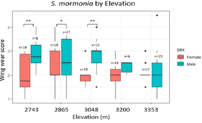
3353 meters (p=0.0017). Average wing wear scores were also greater in males compared
to females (Fig 3.2). The differences between the wing wear scores of males and females
at the three lowest elevations were significantly greater than the corresponding
differences observed at the two highest elevations (Fig 3.3), meaning that there was an
effect by the interaction of sex and elevation on average wing wear scores (F4,172=2.604,
p=0.038).
3.1.2 Wing length
The interaction of sex by elevation, wing wear, and collection year were plugged
into a multifactor ANOVA as co-factors and were determined to have significant effects
on average wing length values. Females had greater average wing lengths compared to
25
Figure 3.1: A box plot of average wing wear score as a function of elevation. Data was pooled from 2017 and 2018. Wing wear was most different between the 2865-meter (2.51±0.75) and 3353-meter (2.06±0.59) elevation groups. (F4,172=3.988, p=0.004)
26
Figure 3.3: A box plot of average wing wear scores for male and female S. mormonia as a function of elevation. Butterflies collected from the elevations of 2743, 2865, and 3048 meters had the greatest disparities in average wing wear scores between males and females (p=0.007, p=0.015, and p=9.99E-06, respectively). Data was pooled from 2017 and 2018.
varied across elevations (Fig 3.5), with the greatest disparity occurring at the lowest
elevation (F9,171=7.907, p=9.94e-10). Average wing length also varied between
elevations (Fig 3.6). As wing wear increased wing length decreased (Fig 3.8;
F1,171=53.58, p=9.24e-12), and the butterflies collected in 2018 had smaller average wing
lengths that those collected in 2017 (Fig 3.7; F1,171=4.98, p=0.027). A separate ANOVA
model, with only the interaction between collection year and sex as co-factors, indicated
that the sexual dimorphism between female and male average wing length was greater in
27
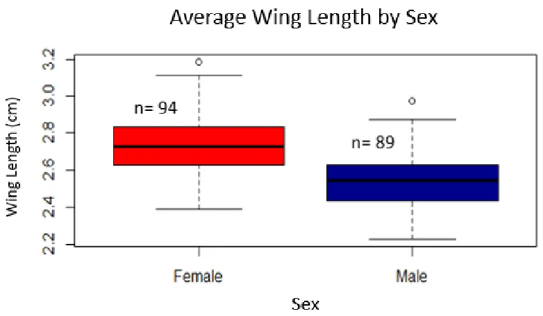
Figure 3.4: A box plot of the average wing length in cm of female versus male S.
mormonia. Wing length data was pooled from both collecting seasons. The average wing length for females (2.73±0.15 cm) was significantly larger than that of males
(2.54±0.16 cm).
3.1.3 Estimated Eye Surface Area
According to a multi-factor ANOVA with sex, year, and wing length as cofactors,
sex and year significantly affected average estimated eye surface area values. Males had
larger average eye surface areas than females (Fig. 3.9; F1,104=52.09, p=8.98e-11). Also,
the average eye surface area for all butterflies was smaller in 2018 than in 2017
(F1,104=18.8, p=3.37e-05). A separate ANOVA demonstrated the significant effect of the
interaction between elevation and sex on average estimated eye surface area data from
2017. Females collected in 2017 tended to have larger eyes at higher elevations, but male
28
Figure 3.5: A box plot representing the average wing lengths of male and female S. mormonia at different elevations. The data came from the 2017 and 2018 field collection seasons. Wing length is more variable in females than males. There are different degrees of female-biased sexual dimorphism in wing length at different elevations, with the greatest dimorphism occurring at the lowest elevation.
3.1.4 Average facet areas
A two-sample t-test revealed that there was an affect by sex on the average facet
areas within particular regions of the eye (Fig 3.11). Males had larger average facet areas
compared to females within regions 1 (t45,0.05=-4.92, p=1.185e-05), 4 (t24.19,0.05=-6.5521,
p=8.578e-07), 5(t45,0.05=-8.2226, p=1.639e-10), 7(t45,0.05=-8.49,p=6.773e-11), and
8(t19.063,0.05=-2.6789, p=0.01482) of the eye. This suggests that males have larger eyes
than females because they have larger facets packed into regions corresponding to the
29
Figure 3.6: A box plot of the average wing length of S. mormonia from different elevations from pooled 2017 and 2018 data. A post-hoc test indicated that the most significant difference in average wing length occurs between butterflies collected at the 2743-meter elevation (2.76±0.22) and those collected at the 3353-meter elevation (2.61±0.15) (p≈0.01).
30
Figure 3.8: A box plot showing average wing length values as a function of wing wear score. The data was pooled from 2017 and 2018. Wing wear is negatively related to wing length.
Figure 3.9: A bar graph showing the average wing length of male and female S. mormonia by year of collection. There seems to be a greater disparity between the
31
Figure 3.10: A box plot showing the average estimated eye surface area for male and female S. mormonia. This data was pooled from 2017 and 2018. The average estimated eye surface area of males (2.95±0.6 mm2) was significantly larger than that of females (2.82±0.4 mm2).
Figure 3.11: A box plot showing the average estimated eye surface areas of butterflies collected in 2017 and 2018. The average estimated eye surface area of butterflies
32
3.1.5 Rhabdom length
A two-sample t-test revealed that male S. mormonia have longer average rhabdom
lengths than female conspecifics, especially in the frontal and dorsal regions of the eye
(Fig 3.12). A total of 8 cryosections from 5 male and 9 cryosections from 6 female eyes
were used to measure rhabdom length. In our sample population, rhabdom length ranged
from 379±19 to 481±15 𝜇m in males, and from 316±18 𝜇m to 394±30 𝜇m in females.
The overall average rhabdom length was 437±1 𝜇m in males and was significantly
greater than the average rhabdom length in females, which was 353±3𝜇m (t15,0.05=-3.67,
p= 0.0023).
Figure 3.12: A box plot showing the average estimated eye surface area data from the 2017 field season plotted separately for males and females, across elevations. In a
33
3.1.6 Relationship between eye size and wing length
Using a Pearson regression analysis on RStudio, I found that only butterflies
collected from the first field season showed a statistically significant, slight negative
correlation between eye surface area and wing length (Fig 3.13). No such correlations
existed between the two variables in butterflies collected during the second field season.
Figure 3.13: A bar graph showing the average facet areas for male and female S. mormonia for each region of the eye. I sampled 31 female eyes and 18 male eyes to obtain these results. The average facet areas within region 1 (M: 486±52.1 𝜇m2; F: 419±42.9 𝜇m2), 4 (M:570±64.1 𝜇m2; F: 456±41.8 𝜇m2), 5(M: 563±48.6 𝜇m2; F: 445±43.7 𝜇m2), 7(M: 552±48.1 𝜇m2; F: 437±42.9 𝜇m2), and 8(M: 425±60.8 𝜇m2; F: 387±24.8 𝜇m2) were found to be significantly larger in males compared to females.
3.2 WING COLOR MEASUREMENTS 3.2.1 Dorsal forewing chromaticity
A multi-factor ANOVA analysis with sex, collection year, and wing wear scores yielded
the following results. Average dorsal forewing chromaticity values were greater in males
34
the 2018 field season compared to those collected in the 2017 field season (Fig 3.15;
F1,100=28.392, p=0.000). Average dorsal forewing chromaticity also decreased as wing
wear increased (Fig 3.14; F5,100=6.008, p=0.000).
Figure 3.14: A bar graph showing the average rhabdom lengths of male and female S. mormonia for the dorsal, frontal and ventral regions of their eyes. I sampled 8
cryosections from 5 male eyes and 9 cryosections from 6 female eyes to obtain these results. The average rhabdom length of males was larger than that of females in every eye region tested, with statistical significance at the dorsal (t15,0.05=-2.4, p=0.0296) and frontal regions of the eye (t15,0.05=-4.69, p=0.0003).
3.2.2 Dorsal hindwing Chromaticity
A multifactor ANOVA analysis with year and wing wear as co-factors showed the
35
collected in 2018 compared to those collected in 2017 (Fig 3.18; F1,105=5.644, p=0.0193)
and decreased as wing wear increased (Fig 3.17; F1,105=5.676, p=0.019).
Figure 3.15: A scatterplot showing the negative relationship between wing length and eye surface area values from the dataset corresponding to the 2017 field season (r=-0.2).
36
Figure 3.17: A box plot showing the average dorsal forewing chromaticity by year of collection. The average dorsal forewing chromaticity from the butterflies collected in 2018 (0.17±0.05) is greater than those collected in 2017 (0.13±0.05).
37
Figure 3.19: A boxplot showing average dorsal hindwing chromaticity values plotted against wing wear scores. Dorsal hindwing chromaticity has a negative relationship to wing wear score.
Figure 3.20: A box plot of the average dorsal hindwing chromaticity values of butterflies collected in 2017 and 2018. The average dorsal hindwing chromaticity was greater for the butterflies collected in 2018 (0.19±0.06) than for butterflies collected in 2017
38
3.3 COMPUTATIONAL MODEL OF VISUAL SENSITIVITY 3.3.1 Results from the electroretinography trials
The data points composing the MoR curve represent the absolute value of the
difference between the highest and lowest voltage responses of eyes from S. mormonia
for each wavelength (from 400 to 700 nm). The shapes of the response curves of male
and female S. mormonia were similar, so I averaged the data from both sexes to create an
MoR curve, which estimates spectral sensitivity (Fig. 3.19). A long-wavelength visual
pigment with a peak wavelength of absorbance of 550 nm was a poor fit for the
long-wavelength tail of the MoR curve, despite the long-long-wavelength visual pigment of
Speyeria leto having a wavelength of peak of absorbance of 550 nm (Yuan et al. 2010).
When I changed the peak wavelength of absorbance to 570 nm instead, the
long-wavelength sensitive pigment absorbance curve was a better fit for the MoR curve (Fig
3.20) Therefore, I used both the 550 nm and 570 nm wavelengths as absorbance maxima
corresponding to the long-wavelength sensitive visual pigment curve in the
computational model. I also compared how these differences in lambda max values of the
long-wavelength sensitive visual pigment affected the resulting ∆St output values. Since I
only exposed the butterflies to wavelengths of 400-700 nm, it was not possible to
determine whether the short-wavelength absorbance curve fit the MoR curve produced
from the ERG data. Given that I was only interested in determining the discriminability
of stimuli from dorsal wing regions, which are orange in color, sensitivity to long
39
Figure 3.19: A scatterplot showing magnitude of response (MoR) as a function of wavelength. Data was obtained from DC electroretinography recordings of 3 male and 3 female adult S. mormonia. Responses from male (green) and female (red) butterflies were similar. The pooled data from this MoR curve was used to approximate the wavelengths of peak spectral sensitivity of the visual pigments of S. mormonia.
3.3.2 Results from the Computational Model for Color Discriminability
The results of the computational model indicate that S. mormonia can distinguish
between the hues of orange displayed by the wings of conspecifics. When average reflectance
data corresponding to the dorsal hindwings and dorsal forewings from butterflies collected in the
2017 and 2018 field seasons were applied to the model, the ∆St output values of these models
were all greater than 1. Using different wavelengths of maximum sensitivity (i.e. 550 nm versus
570 nm) for the long-wavelength sensitive visual pigment absorbance data influenced ∆St values
but did not change the outcome of the model. In the models with 2017 and 2018 reflectance data
inputs, setting the webber fraction to 0.01 and the wavelength of maximum sensitivity to 570 nm
0 0.1 0.2 0.3 0.4 0.5 0.6 0.7 0.8 0.9 1
400 450 500 550 600 650 700
Ave rag e N o rm ali zed M ag n itu d e o f Respo n se (M o R )
Wavelength (nm)
Magnitude of Response Curve for
S. mormonia
female male pooled
40
generally yielded larger ∆St values (Table 3.1 and 3.2).
Figure 3.20: A pigment absorbance template (Stavenga et al.1993) with maximum sensitivity peaks at 385 (purple), 470 (blue), and 570 nm was used to obtain the pigment absorbance curves corresponding to the short-, middle-, and long-wavelength sensitivity visual pigments. These are plotted alongside the MoR curve. When the absorbance of the long-wavelength sensitive pigment has its maximum sensitive wavelength set to 550 nm (black dotted curve), which was determined to be the peak wavelength of sensitivity for one Speyeria leto female, the long-wavelength sensitive curve was to the left of the MoR data curve. However, changing the long-wavelength sensitivity peak to 570 nm (solid green) instead shifted the absorbance curve closer to the MoR curve. Therefore, 570 nm was also plugged into the computational model as a maximum absorbance peak.
The ∆St output values indicate that males have more perceivable variations in
wing reflectance than females and that these variations in male wing reflectance are
discriminable by the S. mormonia visual system (Figure 3.23-3.24). Models which
compared inter-elevational differences in the average reflectance data from male dorsal
forewings and dorsal hindwings consistently yielded higher ∆St values than the models 0 0.2 0.4 0.6 0.8 1 1.2
400 450 500 550 600 650 700
A ver ag e N or maliz ed M agn it u d e of R esp on se / Pigme n t Ab sor b an ce Wavelength (nm)
Magnitude of Response Curve for
S.
mormonia
pooled UV Blue
41
which compared inter-elevational differences in the average reflectance data collected
from female wings. This trend occurred when reflectance data from both collection
seasons were plugged into the model. This means that the variation in male dorsal
forewing chromaticity and dorsal hindwing chromaticity across elevations are
functionally relevant, because they are perceivable by S. mormonia.
Finally, setting the wavelength of maximum absorbance at 570 nm in the models
generally yielded larger ∆St output values than when 550 nm was used as the sensitivity
peak of the long-wavelength visual pigment. This may indicate that S. mormonia has
greater spectral sensitivity at higher wavelengths, which may allow S. mormonia to
distinguish between hues of orange that related butterflies, like Dryas iulia or Speyeria
leto, may not be able to distinguish between. However, follow up studies are needed to
corroborate this observation.
Table 3.1: Color discriminability values (∆St) corresponding to comparisons between the average male and female dorsal hindwing reflectance spectra from 2017 and 2018
Table 3.2: Color discriminability values (∆St) corresponding to comparisons between the average male and female dorsal forewing reflectance spectra from 2017 and 2018
wavelengths of max. sensitivity Collection Year λ max=550nm λ max=570nm
2017 ΔS=6.87 ΔS=7.66
2018 ΔS=6.25 ΔS=6.7
wavelengths of max. sensitivity Collection Year λ max=550nm λ max=570nm
2017 ΔS=5.72 ΔS=6.36
42
Figure 3.23: A bar graph showing the ∆St output values of computational models
comparing the average reflectances from males versus females from different elevations in the 2017 field season. The difference between the average reflectances of dorsal forewings and dorsal hindwings of males versus females were both discriminable. Two-sample t-tests demonstrated that the ∆St value corresponding to the models comparing inter-elevational differences between male dorsal hindwing and dorsal forewing average reflectances were significantly larger than the ∆St output values of models comparing corresponding inter-elevational stimuli in females (dorsal hindwing: t4,0.05=2.78 and p=0.0003; dorsal forewing: t4,0.05=2.78 and p=0.0001). Also, the inter-sexual differences of dorsal hindwing and dorsal forewing average reflectances are greater on butterfly wings collected from low elevation sites than in those collected at high elevation sites (dorsal hindwing: t4,0.05=2.78 andp=4.55E-06; dorsal forewing: t4,0.05=2.78 and
p=0.0003). 0 5 10 15 20 25 30
Avg. M&F 9kM&9kF 11kM&11kF 11k-9k F 11k-9k M
Color Dis crim in ab ili ty v alu es ( ∆S t) Stimulus Pairs
Color Discriminability Values Corresponding to Dorsal
Hind-and Fore-wing stimulus pairs from 2017 Field-caught
butterflies (
𝜔
=0.01)
43
Figure 3.24: A bar graph showing the ∆St values corresponding to the comparison of dorsal hindwings and forewing reflectance data from male versus females of different elevations from the 2018 field season. Two-sample t-tests revealed that the ∆St values corresponding to the models comparing inter-elevational differences between male dorsal hindwing and dorsal forewing average reflectances were significantly larger than the ∆St output values of models comparing corresponding inter-elevational stimuli in females (dorsal hindwing: t5,0.05=2.57 andp=0.000422; dorsal forewing: t4,0.05=2.78 and p=2.99E-05). Also, the intersexual differences of dorsal hindwing and dorsal forewing average reflectances are greater on butterfly wings collected from high elevation sites than in those collected at low elevation sites (dorsal hindwing: t4,0.05= 2.78 and p=2.88E-08; dorsal forewing: t4,0.05= 2.78 and p=3.15E-06, respectively).
0 5 10 15 20 25 30
Avg. M&F 9kM&9kF 11kM&11kF 11k-9k F 11k-9k M
Color Dis crim in ab ili ty ( ∆S t) Stimulus Pairs
Color Discriminability Values corresponding to Dorsal
Hind- and Fore-wing stimulus pairs from 2018 Field
Collected Butterflies (
𝜔
=0.01)
44 CHAPTER 4
DISCUSSION
4.1 Sex-specific energy investment strategies between male and female S. mormonia in response to resource-dependent shifts across elevations
Overall, the data corresponding to morphometric parameters (i.e. wing length and
eye size) for these study populations of S. mormonia suggest that this species may have
sex-specific energy investment strategies in response to the local energy resources which
are available to them. Females consistently had longer wings than males (Fig 3.5). This
is a typical sexual dimorphism observed in S. mormonia (Boggs 1987). Longer wings in
females have been linked to a greater success in egg-laying ability, because this allows
females to maintain flight performance as they carry heavy egg-loads during oviposition
(Turlure et al. 2016). Males had larger eyes than females (Fig 3.9); this was consistently
true at all elevations. This was partly because males had larger facets within regions 1, 4,
5, 7 and 8 of their eyes (Fig 3.11) and longer rhabdoms compared to females (Fig 3.12).
Visual sensitivity increases as rhabdoms get longer and facets get wider (Land and
Nilsson 2012). Therefore, the males likely have greater visual acuity and sensitivity than
females, especially in the frontal, ventral, and dorso-medial regions of the eye,
presumably to optimize their ability to find mates. This finding is consistent with
observations made of other patrolling species of butterflies such as Boloria aquilonaris or
45
mate-seeking strategy may benefit from having acute zones located along the frontal and
ventral regions of the eye, as females usually appear in front of or beneath them
(Rutowski 2000). This is different than species with perching males, like Pararge
aegeria or Coenonympha pamphilus, wherein males benefit from having frontal and
dorsal acute zones because females fly in front of or on top of them while they sit and
wait (Rutowski 2000).
These sexually dimorphic traits in S. mormonia may be linked to sex-specific
constraints of nitrogen consumption during larval development (Carol Boggs, personal
communication). Therefore, the fact that males develop larger eyes compared to females
while females develop larger wings may suggest that males are optimizing mate-seeking
ability strategies while females optimize egg-laying rates and fecundity (Turlure et al.
2016). Both investment strategies, though different, may be predicted to increase the
reproductive fitness of members in this species. Further, these sexually dimorphic traits
may impact traits relevant to visual ecology by causing modifications to the quality of the
visual signal (i.e. wing length) and to the visual system (i.e. eye size).
I expected to see larger butterflies at higher elevations because the temperature
size rule and Bergmann’s law predict that organisms should have larger body sizes (i.e.
wing lengths) at colder temperatures, which are usually associated with higher elevations
(Angilletta Jr. et al. 2003). However, S. mormonia from these sample populations showed
cross-elevational wing length patterns consistent with the converse Bergmann’s law
instead (Mousseau 1997): butterflies had shorter wings at higher elevations instead of
lower elevations. More importantly, there was an effect of sex in the average wing length
46
average wing length values was generally greater at lower elevations. The degrees of
sexual size dimorphism observed in the estimated eye surface area values from the
dataset collected in 2017 (Fig 3.12) and in the average wing length values from the
pooled data set (Fig 3.9) were generally more extreme at lower elevations compared to
higher elevations. These results resemble those of a study which investigated how
morphometric parameters changed in species of grasshoppers along an elevational
gradient (Laiolo et al. 2013). The sexual size dimorphism displayed by the grasshoppers
was less extreme at higher elevations. This has been linked to shifts in climatic features
from one elevation to the next, particularly precipitation and temperature. It seems that
male and female grasshoppers reacted differently to variations in their environment.
Since precipitation and temperature, which directly impact the abundance of host plants,
both tend to decrease at higher elevations, female grasshoppers were largest (relative to
males) at low elevations in comparison to high elevations. This is because female
grasshoppers showed greater plasticity than males in response to increases in host plant
abundance. Overall, these disparities in sexual size dimorphisms across elevations have
also been shown to apply to many other species of insects as well and seem to be a
by-product of sex-dependent responses to changes in local environmental conditions (Tedder
and Tammaru 2005; Nylin and Svard 1991).
My results suggest that male S. mormonia invest in making larger eyes that may
be associated with better vision, whereas females invest in making larger bodies (i.e.
longer wings). In this case I predict that the environmental factor to which S. mormonia
areresponding may be larval host plant abundance. S. mormonia are relatively
47
most of their nitrogenous amino-acid compounds from the leaf-based diets consumed in
their larval state. Females may have longer wings than males, in part, because they spend
relatively more time consuming host plant than males do in the larval stage as a result of
protandry (Boggs 1987). This is reinforced by the fact that female S. mormonia have
significantly greater body masses in pupation and eclosion than males do (Boggs 1987;
Karlsson 1994), which is directly related to the degree of larval host plant intake (Carol
Boggs, personal communication). Moreover, the way in which S. mormonia redistribute
their body mass in adulthood occurs in a sex-specific manner which reinforces the
suggested presence of sex-specific energy investment strategies in this species (Karlsson
1994). At eclosion, females have greater abdomen to total body mass ratios while males
have greater thorax to total body mass ratios. Since they cannot feed on pollen to
supplement their larval diet, both male and females lose body mass over time, but the rate
at which males lose body mass is much slower than females, especially at the thorax
region. Females also redirect the body mass at the thorax to their abdomens over time to
optimize egg-laying success despite their nitrogen-limited adult diet (Karlsson 1994).
This is likely the case because males need energy in their flight muscles, which are in the
thorax, to patrol for mates, while females need more fat reserves in their abdomens to
optimize egg-laying success.
Therefore, this sex-specific energy investment strategy of S. momornia seems to
be characterized by the following: females spend a longer time in the larval stage feeding
than males do as a result of protandry, which causes them to eclose with larger body sizes
(i.e. wing lengths) in comparison to males (Boggs 1987). The later emergence in females