Tweets About Tornado Warnings: A Spatiotemporal And Content Analysis

(1)

University of South Carolina

Scholar Commons

Theses and Dissertations

2018

Linking Microbial Phylogenetic and Functional

Gene Diversity to Microbial Mat Ecosystem

Function Following Environmental Disturbance

Eva Christine Preisner

University of South Carolina

Follow this and additional works at:https://scholarcommons.sc.edu/etd Part of theEnvironmental Health Commons

This Open Access Dissertation is brought to you by Scholar Commons. It has been accepted for inclusion in Theses and Dissertations by an authorized administrator of Scholar Commons. For more information, please [email protected].

Recommended Citation

(2)

LINKING MICROBIAL PHYLOGENETIC AND FUNCTIONAL GENE DIVERSITY TO

MICROBIAL MAT ECOSYSTEM FUNCTION FOLLOWING ENVIRONMENTAL

DISTURBANCE

by

Eva Christine Preisner

Bachelor of Science

University of Duisburg-Essen, 2010

Master of Science

University of South Carolina, 2012

Submitted in Partial Fulfillment of the Requirements

For the Degree of Doctor of Philosophy in

Environmental Health Sciences

The Norman J. Arnold School of Public Health

University of South Carolina

2018

Accepted by:

Robert Sean Norman, Major Professor

Alan W. Decho, Committee Member

Anindya Chanda, Committee Member

James Pinckney, Committee Member

(3)

ii

(4)

DEDICATION

This work is dedicated to the beautiful microbial mats on San Salvador Island,

The Bahamas that have gained, besides the attention from scientists, little

acknowledgement from the general public and locals who have called the Ponds

(5)

iv

ACKNOWLEDGEMENTS

This work could not have been done without the help of many people. First and

foremost I want to acknowledge my family in U.S. and back home in Germany, who

supported me in many ways. Especially my husband who has been there for me and

always had an open mind to discuss my research, sat through plenty of practice talks, and

motivated me to keep going when I wanted to give up. My son, the light of my life, who

put things in perspective the moment he was born. A great thank you to all my other

grad-student friends who can easily relate to the hard work of being in graduate school

and who always supported me. My lab peers have been wonderful throughout the years

and helped me develop into a better scientist by teaching me new methods and discussing

research. A special acknowledgement to Erin Fichot and Gargi Dayama who both were

not only my lab mates but became my closest friends. The people from the RCI, Paul,

Nathan, and Ben at the University of South Carolina were more than supportive of our

lab and helped us tremendously with the computational resources to handle the

bioinformatics side of our research. A special thank you to Ben Torkian, who did not

mind my endless questions and quickly wrote an R or Phython script for me to help with

the analysis. I also want to thank Dr. Jay Pinckney’s lab group for helping me with

sample preparation and photopigment analysis. I am very grateful to have Dr. Pinckney

on my doctoral committee; he always had an open door to talk about my research and the

sample site, and was a great help with statistical analysis. I want to give a special

(6)

doctoral committee. To the last member of committee Dr. Alan Decho, for helping us

with this study by sharing knowledge and lab equipment. I also want to thank everyone

we have worked with and all the staff at the Gerace Research Station on San Salvador

Island, the Bahamas; we certainly couldn’t have done all the research without their help.

Lastly, I want to give a big thank you to my adviser and mentor Dr. Sean Norman, who

invited me to come study in his lab and didn’t let me go until I had my PhD, it has been a

(7)

vi

ABSTRACT

The ability of ecosystems to adapt to environmental perturbations depends on the

duration and intensity of change and the overall biological diversity of the system. In this

study, a microbial mat ecosystem located on San Salvador Island, the Bahamas was used

as a model to examine how environmental disturbance affects microbial community

resistance, their protein synthesis potential (PSP), ecosystem function as measured by

biogeochemical cycling, community stability, and resilience. This ecosystem experienced

a large shift in salinity (230 to 65 g kg−1) during 2011–2012 following the landfall of Hurricane Irene on San Salvador Island. High throughput sequencing and analysis of 16S

rRNA and rRNA genes from samples before and after the pulse disturbance showed

significant changes in the diversity and an increase in PSP of abundant and rare taxa,

suggesting overall compositional and functional sensitivity to environmental change.

Together, these findings show complex community adaptation to environmental change

and help elucidate factors connecting disturbance, biodiversity, and ecosystem function

that may enhance ecosystem models. Based on these findings, a long-term study was

conducted to answer questions about the impacts of seasonal and pulse disturbance on the

community resistance, ecosystem function and stability, and resilience using a

comparative metagenomic approach. Over the course of four years the microbial mat

community was monitored and vertical sections were taken at eight time points. We

found that a wide range of environmental factors play a role in shifting the

(8)

vertical niche differentiation within the mat. Community composition did not

significantly change on Archaea and Bacteria phyla level but on class level. The

microbial community of the deepest layer was resistant to environmental disturbance,

while upper layers changed in community composition and did not return to its

pre-disturbed state, suggesting that the community was not resilient to the disturbance event

after one year. Assessing apparent functional capacity of the archaeal metagenomes over

time showed that the metagenome of the first three time points were distinct from all

(9)

viii

LIST OF TABLES

Table 1.1 An ecological guide to avoid confusion ...21

Table 2.1 Metadata of Salt Pond collected at day and night ...35

Table 2.2 Photosynthetic active radiation (PAR) lost in water column ...35

Table 2.3 O2 Productivity at 0.2 mm depth ...35

Table 2.4 Photopigments found in site 1 and 2 microbial mats ...35

Table 3.1 MID sequences added to the U529 reverse primer ...70

Table 3.2 qPCR Primers for genes involved in biogeochemical processes ...71

Table 3.3 Comparison of pre- and post-disturbance mean PSP ...72

Table 3.4 Archaea class summary of OTUs ...72

Table 3.5 Bacteria class summary of OTUs ...73

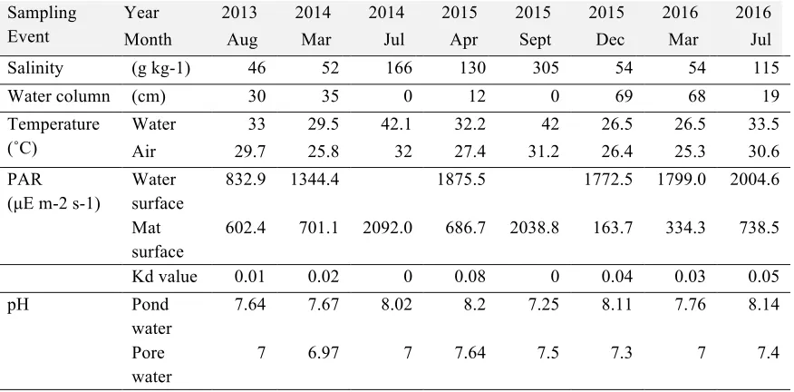
Table 4.1 Metadata collected at each time point from Salt Pond sampling site ...125

Table 4.2 α-diversity measured between the different layers of the microbial mat ...126

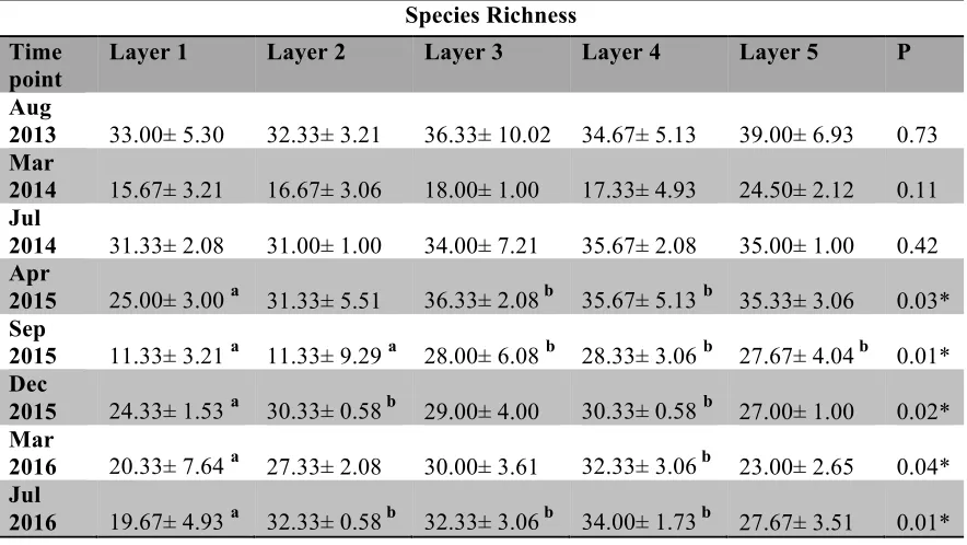
Table 4.3 Species Richness of microbial mat layer by layer ...126

Table 4.4 Metagenome assembly of all time points of the study classified by lineage ...127

Table 4.5 Metagenome assembly of all time points of the study: Archaea phyla ...127

Table 4.6 Metagenome assembly of all time points of the study: Bacteria phyla ...128

Table 4.7 Metagenome assembly of all time points of the study: Eukaryota phyla ...129

Table 4.8 Metagenome assembly of all time points of the study: Virus phyla ...129

Table 4.9 Metagenome assembly of all time points of the study: Proteo class ...130

(12)

Table 4.11 Summary of Bbmap quality report ...131

(13)

xii

LIST OF FIGURES

Figure 1.1 The intermediate disturbance hypothesis by Connell (1978) ...22

Figure 1.2 Vertical cross sections of microbial mat from different environments ...22

Figure 1.3 A generalized biosphere model of basic inputs and outputs of energy and materials ...23

Figure 1.4 Schematic of the microbial nitrogen cycle ...23

Figure 1.5 Biogeochemical cycling in microbial mats ...24

Figure 1.6 Workflow of common metagenomic analytical strategies ...25

Figure 2.1 Representative surface and cross sections of microbial mats in March 2013 in Salt Pond ...36

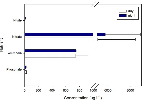
Figure 2.2 Nutrient analysis in Pond water at midday and midnight ...37

Figure 2.3 Representative oxygen depth profiles taken with microsensor (unisense) of microbial mats on site 1(far shore, blue) and 2 (near shore, green) ...37

Figure 2.4 Comparison of photopigments detected in Salt Pond microbial mats of sites 1 and 2 ...38

Figure 3.1 Overview of Sample Site ...74

Figure 3.2 Non-parametric multidimensional scaling (NMDS) plots ...75

Figure 3.3 Stacked bar charts of microbial mat community profiles for Archaea (A) and Bacteria (B) ...76

Figure 3.4 Relationship between rRNA and rDNA abundance for each OTU ...77

Figure 3.5 Heatmap analysis of OTU PSP for each archaeal class for day and night ...78

Figure 3.6 Heatmap analysis of OTU PSP for each bacterial phylum for day and night ..79

(14)

Figure 3.8 Microbial mat community potential for biogeochemical cycling ...81

Figure 4.1 Overview of workflow implemented ...133

Figure 4.2 Photos of Salt Pond Sample side and microbial mats ...134

Figure 4.3 Dissolved oxygen concentrations ...135

Figure 4.4 Dissolved organic carbon (DOC) concentrations ...136

Figure 4.5 Nutrient concentrations in Salt Pond ...137

Figure 4.6 Microbial community composition over the course of the study ...138

Figure 4.7 NMDS ordination plot of Bray-Curtis community dissimilarities ...139

Figure 4.8 Beta diversity analysis of taxonomic classification based on class level ...140

Figure 4.9 Krona graphical representation of the relative percentage of bases from the assembly belonging to the different lineages ...141

Figure 4.10 Archaea lineage: Breakdown of bases from assembly ...142

Figure 4.11 Bacteria lineage: Breakdown of bases from assembly ...143

Figure 4.12 Prodigal called genes (amino acid sequences) from overall archaea metagenomic assembly ...144

Figure 4.13 Prodigal called genes (amino acid sequences) from overall bacteria metagenomic assembly ...145

Figure 4.14 Microbial mat community potential for biogeochemical cycling ...146

Figure 4.15 Analysis of variance comparison of Archaea assigned COG categories between time points ...147

Figure 4.16 Archaea comparison of protein functions based on COG categories in different layers and over time ...148

Figure 4.17 Principal component analysis (PCA) plot comparing functional profiles for Bacteria between time points ...149

(15)

xiv

Figure 4.19 Archaea comparison of protein functions based on COG categories in

(16)

CHAPTER 1 INTRODUCTION

1.1 Ecosystem Ecology

The term ”ecosystem” was first defined by Sir Arthur Tansley in 1935 as a biotic

community or assemblage, including its physical (abiotic) characteristics, located in a

specific place. There are three major facets to an ecosystem. First, an ecosystem includes

the interactions between the biotic community, which can consist of any forms of living

species (e.g. animals, plants, microbes, etc.), and the abiotic factors that demonstrate the

physically unique environment in a given place (e.g. temperature, salinity, UV, pH, etc.

(Tansley, 1935). Second, an ecosystem is scale-independent, meaning it can be of any

size so long as organisms, their physical environment, and biotic/abiotic interactions can

exist within (Allen and Hoekstra, 1992). Hence, an ecosystem can be small--such as a

microbial mat or a patch of soil--or as large as an ocean. According to (Thiel, 1994)

Likens (1992) and (Odom, 1993), when defining a specific ecosystem, an explicit extent

(area, size etc.) must be specified and bounded. Third, an ecosystem is not restricted by

equilibrium, complexity, or stability (Holling, 1973), meaning that it can be dynamic or

in steady state, simple or complex. Tansley’s basic definition of an ecosystem covers an

unimaginably broad array of spatial scales—from microbial to biospheric, temporal

scales—from instantaneous to geological, and disciplines--from biodiversity to evolution

(Jones C. G. 1995). Identifying a changing ecosystem can be difficult, so (Rykiel, 1985)

(17)

2

stress, perturbation or disturbance). The reference state determines the significance of

those changes, including some measure of biological and ecological impact on the

system. There are two proposed ways to define a reference state. First, the reference state

can be the system’s steady state which is defined under optimal conditions (idealization),

or secondly, the reference state can be the current state of the system despite its dynamic

status. Based on the reference state, ecosystem change can be quantified and seen in

terms of cause (disturbance) and effect (perturbation).

It is often understood that disturbances initiate ecosystem change through damage

or destruction to the system (e.g. wildfire) after which the system has to recover to reach

the initial reference state (Bazzaz 1983). However, the intermediate disturbance

hypothesis (IDH) by Connell (1978) states that disturbances can improve ecosystem

stability. Specifically, the hypothesis has 2 parts: 1) a “disturbance of a certain intensity

and frequency may prevent one or a few species from dominating resources” and 2) a

disturbance is “not so biologically damaging that only a few species can use the resulting

resources” (Connell 1978). He suggests that the highest number of different species

(highest richness) will be reached at intermediate level of disturbance (Figure 1.1) and

that both high and low levels of disturbance would lead to reduced diversity. According

to his hypothesis, diversity will decline if disturbances are infrequent and of low

intensity. But at intermediate levels of disturbance there is enough time between

disturbances for a wide variety of species to colonize but not enough time to allow

competitive exclusion. Those ecological community changes following a disturbance are

termed succession. There are three distinguishable types of successions: 1) primary and

(18)

pre-existing communities and is then newly colonized is termed primary succession. 2)

Secondary succession is started by an event (disturbance) and reduces the already

established ecosystem to smaller population of species (Bard 1952). 3) Cyclic succession

can be described as a state where major disturbances are absent and is driven by pattern

of smaller scale changes in which a smaller number of species replaces each other over

time (Morin 1999). Climate cycles for example can result in cyclic successions by

directly altering physical changes (Glenn-Lewin 1992).

Connell’s IDH predicts that in early successional stages, disturbance leads to

reduction in diversity. Overall, the IDH has been a topic of many studies and appears in

ecological textbooks (Ricklefs 1999; Begon 2005; Lampert 2007); however, 100

published empirical studies as reviewed by Mackey and Currie (2001) show that the peak

in diversity at intermediate disturbance levels hardly occurs (< 20% of studies), a result

corroborated in another review published in 2007 by Hughes et al. (2007). In Fox’s

(2013) opinion, the IDH should be “abandoned”. He argues that it is theoretically invalid

and most of the time can not be explained by empirical data. However, models that were

developed recently predict various diversity–disturbance relationships, including different

shaped relationships (Miller et al. 2011). That is why Fox suggests focusing on testing the

assumptions and predictions of logically valid models of diversity and coexistence in

fluctuating environments.

Definitions for resilience and stability of ecological systems are challenging and

depend highly on how one defines equilibrium of a system. Ecological stability concepts

are very diverse in the literature (for more information see review of 163 definitions of

(19)

4

different categories for the definition of stability: (1) “staying essentially unchanged”, (2)

“returning to the reference state after a temporary disturbance” and, (3) “persistence

through time of an ecological system”. While definitions of the category 1 are based on a

specific reference state, category 3 is founded on the question of whether a system

persists as an identifiable entity (Shrader-Frechette, 1993; Grimm and Wissel, 1997).

In the literature, resilience reflects different aspects of stability (Holling, 1973, 1996;

Ludwig et al., 1996). Holling (Holling, 1996) defines stability as the persistence of a

system near or close to an equilibrium state (Walker et al. 2004). In other words, stability

quantifies the extent to which a community “stays the same” over a long period of time

(depending on the time scale) or during some disturbances. Resilience, however, is how

far a system has moved from equilibrium state and how quickly it returns (Walker 1981).

However, other sources describe the return times as a measure for stability Holling

(Holling 1973). Walker and Holling state that resilience involves the following four

aspects: latitude, resistance, precariousness, and panarchy (Walker et al. 2004). Latitude

of systems is the maximum amount of disturbance a system can deal with before losing

its ability to recover. Resistance describes how easy or hard it is for the system to change.

Precariousness explains in which state the system is and how close it is to a limit or

“threshold.” Panarchy explains how latitude, resistance, and precariousness are

“influenced by the states and dynamics of the systems at scales above and below the scale

of interest.” A guide to avoid terminological confusion was published by Grimm and

(20)

According to Pielou (1966), diversity refers to the number of species (species richness) or

to a diversity index based on the number of species weighted by relative abundance

(species evenness). The most widely used diversity index is Shannon-Weaver (H’):

H’= - Ʃpi ln pi

where i=species, and p=proportion of total cover (Shannon 1949). Whittaker

(1972) defined three levels of diversity, alpha, beta, and gamma diversity. Alpha diversity

describes the diversity within a particular area or ecosystem, and is usually expressed by

the number of species (e.g. species richness) in that ecosystem. The difference in species

diversity between two ecosystems is a measure of beta diversity; specifically, the total

number of species unique to each of the ecosystems is compared. Gamma diversity

measures the overall diversity for the different ecosystems within a region

("landscape-level" diversity).

Many diversity studies focus on eukaryotes, but it is critical to understand the

patterns of prokaryotic (bacteria and archaea) biodiversity due to the following reasons:

1) bacteria and archeaea display the majority of the Earth’s species diversity and 2) they

are involved in the most important environmental cycles that sustain life on Earth. In

plant- and animal- dominated systems, primary productivity is thought to be the major

determinant for species diversity (Rosenzweig, 1999) The following studies showed that

link in prokaryotes in field systems as well (Benlloch et al., 1995; Øvreås and Torsvik,

1998; Schäfer and Muyzer, 2001; Claire Horner-Devine et al., 2003). In vitro studies

(21)

6

2000) so that the IDH is valid for bacterial systems in lab settings. However, in field

studies, it was shown that bacterial community composition and diversity may respond to

gradients in disturbance (Müller et al., 2002), but it is difficult to assess the applicability

of the intermediate-disturbance hypothesis to bacteria outside the laboratory (Fierer et al.,

2003).

High-throughput sequencing has broadened our understanding of the scope of

biodiversity in ecological systems Sogin et al. (2006). Using operational taxonomic units

(OTUs), an abundant species has been defined as a microorganism with sequences

comprising more than 1% of the sequencing effort (Pedrós-Alió, 2006). Likewise, rare

species have been defined as OTUs representing 0.1% to <1% of the sequences in a

sample (Fuhrman, 2009). The rare biosphere and its functions in ecosystems are mostly

undiscovered. Two main hypotheses have been proposed to explain its role. The first

hypothesis states that the rare biosphere stays inactive and in low abundance until

environmental conditions change, suggesting that the rare biosphere acts like a “seed

bank” (Brown and Fuhrman, 2005; Pedrós-Alió, 2006). The second hypothesis claims

that rare taxa are active and well adapted to their environmental niche and play a role in

ecosystem function (Galand et al., 2009). However, both hypotheses have not been well

tested. The rare biosphere might not be as large as previously believed due to the findings

of methods for error correction in metagenomic sequencing datasets by Reeder and

Knight (2009) . It has also been suggested that the rare biosphere has a biogeography and

that it might be subjected to ecological processes such as selection, speciation, and

(22)

1.2. Photosynthetic Microbial Mats

Microbial mats are complex, densely, layered microbial communities (Stal et al.,

1985). Different types of microbial mats can exist almost all over the world in places

such as marine intertidal and sub tidal zones and in fresh water rivers and lakes, but

microbial mats are mostly found under extreme conditions such as, hot springs, saline

lagoons, hypersaline ponds (Des Marais, 1990) (Figure 1.2). In this study we focus on

microbial mats in hypersaline ponds on San Salvador Island (The Bahamas) (Figure 1.2

B). Physical characteristics that impact the type of organisms in the mat include,

temperature, water content, and flow rate; while chemical characteristics such as pH,

alkalinity, oxidation reduction potential (E0), and concentration of different chemical

compounds (e.g. salts, oxygen, hydrogen sulfide, nitrate etc., as well as organic carbon)

can also impact the microbial mat. In general, microbial mats are self-sustaining

communities that take part in all major biogeochemical cycles and are believed to be

analogous to some of the earliest communities on Earth (Cohen et al., 1989). The

complex community structure fulfills the definition of an ecosystem because there are

interactions between biotic and abiotic elements in a particular space but more

importantly due to the presence of all trophic levels (primary producers, consumers,

decomposers). Nematodes and diatoms are eukaryotes that are usually found in microbial

mats but the eukaryotic diversity in mats is lower than prokaryotic depending on

environmental conditions (Nübel et al., 1999; Feazel et al., 2008).

Due to the unique layered structure of microbial mats, it was thought that each of

(23)

8

et al., 1984). However, when sulfate reducing bacteria (SRB) typically associated with

anoxic layers, were found at the surface level of mats (Canfield and Des Marais, 1991),

this view had to be revised. Mat microorganisms can be classified into six major

functional groups: oxygenic phototrophs, anoxygenic phototrophs, aerobic heterotrophic

bacteria, fermenters, anaerobic heterotrophs, and sulfide oxidizing bacteria (van

Gemerden, 1993; Visscher et al., 1998; Visscher and Stolz, 2005).

Primary producers (e.g. cyanobacteria) belong to the first functional group of the

system (light induced CO2 and N2 fixation) (Paerl et al., 2001). Filamentous

cyanobacteria trap and bind sediment and sand grains together with extracellular

polysaccharide (EPS), thus establishing the foundation for microbial mats. Primary

producers use photosynthetically active radiation (PAR = 400–700 nm), which has been

found to penetrate the first two mm of the mat, in oxygenic and anoxygenic

photosynthesis. The second functional group, anoxygenic phototrophs (e.g. purple and

green bacteria), is also involved in photosynthesis but it uses HS- instead of O2 as an

electron donor. The aerobic heterotrophic bacteria gain energy from respiration of oxygen

and organic carbon and can exist in the range of near infra-red radiation (NIR = 700–

1100 nm) which is deeper in the mat than PAR (van Gemerden, 1980). Using organic

carbon or sulfide compounds as electron donor and acceptor, fermenters build the fourth

functional group (Bak and Cypionka, 1987; Visscher et al., 1999). The fifth group

consists of anaerobic heterotrophs, predominantly SRB, that respire organic carbon with

sulfate and produce hydrogen sulfide ions (HS-). The last functional group, sulfide oxidizing bacteria (SOB), has many chemolithoautotrophs that oxidize reduced sulfur

(24)

groups can be found in microbial mats, however, they are mainly photosynthetically

driven systems and are mostly dominated by cyanobacteria (Stal, 1994).

Photopigments secreted by phototrophic bacteria and archaea result in color

banding visible in depth sections of mats. Diatoms and cyanobacteria are mostly found

in the upper brownish layer. The underlying dark green layer (~2 - 4 mm) has the highest

photosynthetic activity and is dominated by filamentous cyanobacteria such as,

oscillatorians (Microcoleus, Oscillatoria, Lyngbya, Spirulina) and Chroococcales

(Mesrismopedia, Chroococcus) (D’Amelio et al., 1989). All functional groups are

involved in element cycling. Because microbial mats can function with sunlight as energy

input into the system, they can be considered as semi-closed systems(Fenchel, 1998).

These attributes have made microbial mats attractive models for better understanding

elemental cycling, microbial interactions, and the evolution and the ecology of microbial

systems supporting the processes that now sustain our biosphere.

1.3. Biogeochemical cycling in microbial mats

Biogeochemical cycling describes the transport and transformation of substances

(chemicals or molecules) in biotic and abiotic parts of the ecosystem. Microorganisms

play a major role in element cycling (Butcher 1992). In microbial mats, oxygen, carbon,

nitrogen, phosphorous, and sulfur cycles are present and found to be inextricably

interconnected within microbial communities (Canfield and des Marais 1993). For

instance, the oxidation and reduction of nitrogen and sulfur compounds are directly

coupled to the reduction and oxidation of carbon, respectively, all carried out by different

(25)

10

The water in which microbial mats grow is usually nutrient depleted (Javor 1983),

but the mat itself is a highly productive system involved in all major biogeochemical

cycling. Figure 1.3 explains how microbially driven biogeochemical processes are

interconnected based on photosynthesis. The major energy input into the system is sun

light, which triggers both oxygenic and anoxygenic photosynthesis. During oxygenic

photosynthesis, an electron donor, H2O, is oxidized and CO2 fixation occurs ([CH2O]n).

In anoxygenic photosynthesis the electron donors are HS-, H2, or Fe2+ (Figure 1.3).

Electrons and protons from oxygenic and anoxygenic photosynthesis are then used to

reduce inorganic carbon to organic matter. Resulting compounds serve as electron

acceptors in either aerobic/anaerobic respiration or can be used by photosynthetic

organisms (Blankenship et al., 1995).

Phototrophic organisms form the foundation of the carbon cycle, where organic

matter (CH2O) is generated through photosynthesis [CO2 + H2O à (CH2O) + O2]. The

resulting carbohydrates can be degraded in either a respirational or a fermentative

process. Methane and carbon dioxide are formed through the activity of methanogens and

chemoorganotrophs during fermentation, anaerobic respiration or aerobic respiration (see

Figure 1.3). Methane produced in anoxic environments is oxidized to CO2 in the oxic

zone.

In the nitrogen cycle, nitrogen gas fixation is the only biological process that makes N2

accessible for the synthesis of proteins and nucleic acids. N2 is transformed to NH4+, this

reductive reaction is catalyzed by nitrogenase (Figure 1.4, Step 1). Nitrogenase is an

enzyme complex, which is inhibited by oxygen (Postgate, 1998).NH4+ is oxidized to

(26)

pathway by a specific group of Bacteria or Archaea that oxidize ammonia to NO2− (via

hydroxyamine). Nitrifying bacteria then oxidize NO2− to NO3− (Falkowski, 1997) (Step

3). Using the small differences in redox potential in the oxidation reactions, nitrifiers

reduce CO2 to organic matter. Opportunistic microbes are involved in the respiration

pathway that forms N2. Under the anaerobic oxidation of organic matter, NO2− and NO3−

are used as electron acceptors if O2 is absent (Step 4). The nitrogen cycle was believed to

be closed, but research within the last decade found that there are more processes

involved shown in Figure 1.4. step 5 and 6. Step 5 describes both, a process called

anamox where NO is oxidized anaerobically to N2H2 (Strous et al., 1999), and NH4+

oxidation by crenarchaea (Könneke et al., 2005; Francis et al., 2007) as well as the

interaction between these two groups (Lam and Kuypers, 2011). Step 6 shows the

dissimilatory nitrate and nitrite reduction to ammonium (Risgaard-Petersen et al., 2006) .

The sulfur cycle takes place in mostly anaerobic conditions. The major aerobic

process is the oxidation of sulfate to S2- which occurs intracellularly. Organic S

mineralization leads to HS-, which can then be oxidized by oxygen by facultative

chemolithotrophs in a dissimilatory process via O2 or NO3-, Mn4+, or Fe3+ as electron

acceptors. Sulfate is the end product but several intermediates can be found. Sulfide can

also be oxidized in a photosynthetic process resulting in S0 and SO42- (by phototrophic

sulfur bacteria).

Paerl and Pinckney (1996) graphically explained each biogeochemical process

within a depth profile of microbial mats where processes of microbial nitrogen, sulfur and

carbon transformation occur in regard to the biogeochemical transformation take place

(27)

12

ammonia/ammonium (NH4+/NH3) increases (see yellow line shifting more to the right as

oxygen disappears). Nitrification maximizes at oxic/anoxic interface, here

ammonia/ammonium is first oxidized to nitrite (NO2-), which is then oxidized to nitrate

(NO3-). Denitrification is the anaerobic conversion of nitrate to nitrogen (N2) and depends

on high nitrate concentrations within the sediment. N2 is then converted to ammonium via

N2 fixation.

Sulfate (SO42-) concentrations are highest in oxic zone (see yellow line) while in

the anaerobic environment sulfide (S2-) is reoxidized to elemental sulfur (S), sulfate, or

thiosulfate. In the carbon cycle, anaerobic respiration is localized in oxic zone; whereas

anaerobic respiration and fermentation as well as methanogenesis are deeper in the

anaerobic zone.

1.4. Molecular based tools

Several molecular-based tools exist to study ecosystem function, one of which is

the use of transcript analysis. In transcriptomics, the abundance of major genes involved

in elemental cycling are quantified to examine the rate of biogeochemical cycling

occurring at a given time or over time. Using reverse transcriptase quantitative

polymerase chain reaction (RT-qPCR), it is possible to calculate how many copies of the

gene of interest were present at the time of sampling, which helps to estimate up- or

down- regulation of a specific pathway within the microbial mat. To study nitrogen

fixation, researchers can use a part of the nitrogenase pathway, which is encoded by the

gene nifH (the reductase). The gene involved in the process of archaeal and bacterial

nitrification (Step 2 in Figure 1.4.) is called amoA (ammonium monoxygenase). The

(28)

and nosZ). A functional gene that encodes a key enzyme (reductase AprBA) of the

dissimilatory sulfate-reduction pathway can be used to look at the sulfur cycle in sulfate

reducing (SRB) and oxidizing bacteria (SOB). The terminal step of the pathway in

methanogenesis is the expression of methyl coenzyme-M reductase subunit A (mcrA)

gene. This can be used as an indicator of the methanogenic activity (Nazaries et al.,

2013).

Photopigments can be used as a measure of distribution of oxygenic (oxygenic

chlorophyll a (Chl a)) in relation to anoxygenic photosynthesis (bacteriochlorophyll

(BChl)). Both processes together with chemoautotrophy resemble primary production.

According to Stal et al., (1985) primary productivity (especially CO2 fixation) and

nitrogen fixation can be an ecophysiological measure for phototrophic community

growth. Primary productivity can also be a measure of trophic stability and an indicator

of ecosystem recovery after a perturbation (Oksanen et al., 1981). Adenosine

triphosphate (ATP), generated during photosynthesis is used for reproduction and cell

growth, but after a disturbance it can shift towards stress compensating mechanisms in

the cell resulting in lower primary productivity.

There are different approaches to look at the relative abundance of species within

the microbial mat. Depending on the research interest, one can use chemosystematic

photopigments as indicators of the relative abundance when looking at the phototrophic

community of the mat. Analysis of the 16S rRNA genes give information of the total pool

of DNA that might consist of DNA derived from living, dormant or even dead cells as

well as extracellular DNA (Josephson et al., 1993). DNA has a relatively long life span as

(29)

14

metabolically active fraction of the community (Mills et al., 2005; Moeseneder et al.,

2005; Gentile et al., 2006). There is a linear relationship between cellular rRNA content

and the growth rate in bacteria (DeLong et al., 1989; Kemp et al., 1993; Kerkhof and

Ward, 1993). During starvation, the rRNA content decreases to minimum levels in the

cell (Fegatella et al., 1998). The higher amount of rRNA in active than in dormant cells

associated with the higher number of ribosome in active cells provides a tool to determine

the metabolically active members of the bacterial community (Poulsen et al., 1993). To

explore an aspect of activity and dormancy the abundance of the 16S rRNA gene

transcripts is compared to the abundance of bacterial and archaeal communities via 16S

rRNA genes (rDNA). Here we are using the term rDNA when we describe the 16S rRNA

genes to differentiate between transcripts of the gene and the gene itself. The ratio of 16S

rRNA to rDNA is an index of the growth rate for specific taxa in natural communities

(Jones and Lennon, 2010).

1.5. Comparative Metagenomics

Metagenomics is described as the study of microorganisms by sequencing random

pieces of their genomes directly from environmental or clinical samples (Handelsman et

al., 1998; Rondon et al., 2000). Metagenomics require no prior cultivation of individual

isolates or entire communities, as the method is based solely on nucleic acid extraction of

the sample and microbial communities can therefore be studied directly in their natural

state (Schloss and Handelsman, 2005). Taxonomic compositions and metabolic profiles

of the microbial communities inhabiting a specific environment can be studied using

(30)

differences in community structure, diversity and biological function can be identified.

With the decrease in cost and increase in efficiency within the last decade, high

throughput DNA sequencing technologies (or next generation sequencing technologies)

have become a widely-used tool for the study of metagenomes. The term metagenomics

has been falsely applied to studies performing PCR amplification of certain marker genes

and was referred to as “marker gene amplification metagenomics”. Direct sequencing of

a nucleic acid pool is termed “shotgun metagenomics”, as the whole genetic potential of a

sample is being analyzed. Shotgun metagenomics has evolved to address the questions of

“who” is present in an environmental community, “what” they are doing (function-wise),

but also “how” these microorganisms interact to sustain a balanced ecological niche. Post

sequencing processing of metagenomic data poses a challenge, as there are many

different ways to perform analyses each containing certain caveats. Depending on

sequencing technology used different options of post run processing need to be carefully

assessed.

One of the first steps after removing any sequences containing errors or those

sequences not meeting quality criteria (quality control step, Figure 1.6) is the generation

of a metagenomic assembly. During an assembly collinear metagenomic sequences from

the same genome are being merged into a single contiguous sequence (i.e., contig)

resulting in longer sequence reads, which can simplify bioinformatic analysis relative to

unassembled short metagenomic reads. Due to DNA extraction from the sample, whole

protein coding genes as well as full operons are unlikely to be intact but can offer

invaluable functional knowledge about the community. However, in some cases,

(31)

16

genomic composition of uncultured organisms found in a community. An assembly of

shorter reads into genomic contigs and orientation of these into scaffolds is often

performed to provide a more compact and concise view of the sequenced community

under investigation. Depending on the dataset, there are two approaches for creating an

assembly 1) a reference based assembly or 2) a de novo assembly. When following a

reference based assembly protocol, one or more already existing reference genomes can

be used as a “map” for creating contigs. This approach is often used when metagenomes

are taken from extensively studied areas and genomes of closely related organisms are

already in an online reference database. In the case of de novo assembly, no reference

“map” is being used and contigs from the sequencing run are being assembled. This

process is computational extensive but several programs including MetaVelvet-SL

(Afiahayati et al., 2015; Namiki et al., 2012) and Meta-IDBA (Peng et al., 2011) or

MEGAHIT (Li et al., 2015) address previously arising issues. After assembly and quality

control (MetaQuast (Mikheenko et al., 2016)), sequence reconstruction and grouping can

be performed through binning using various tools such as emergent self-organization

maps (ESOM) (Dick et al., 2009), followed by automated gene or regulatory element

prediction of the sequences using Prodigal (Hyatt et al., 2010). Potential protein coding

genes can then be functionally annotated using a reference database such as NCBI’s

maintained “non- redundant” (NR) protein database (NCBI Resource Coordinators, 2017)

using BLASTp (Altschul et al., 1990, 1997). With the resulting data functional

comparative metagenomics is possible and is based on identifying differential feature

abundance (pathways, subsystems, or functional roles) between two or more conditions

(32)

2006; Pookhao et al., 2015). Tools to carry out such comparisons are programs such as

MEGAN (Huson et al., 2007), Parallel-META 2.0 (Su et al., 2014), or STAMP (Parks et

al., 2014).

Using metagenomics data to investigate the taxonomical composition of one or

more samples does not depend on gene-targeted primers or PCR amplification and is

therefore not affected by the biases (e.g. chimera formation) these methods pose. For

taxonomical composition comparison of metagenomes, phylogenetic marker genes such

as the 16S ribosomal RNA genes can be either extracted from the raw sequencing data or

later separated based on a blast search of the cleaned sequences against for instance the

SILVA rRNA database (Figure 1.6). Extraction from the raw sequencing data by

reconstructing 16S rRNA genes through an assembly tool can be done with programs like

REAGO (Yuan et al., 2015), however it needs to be noted that the use of REAGO is

limited to short (~200 bp) Illumina HiSeq reads and does not support longer (>200 bp)

MiSeq sequencing data. The use of reference gene sequences to assemble rRNA genes

from metagenomics data is used by EMIRGE (Miller et al., 2011), this program requires

large numbers of known rRNA genes for the mapping step and may miss remotely related

rRNA genes. When blasting the cleaned sequences against a reference rRNA database

such as SILVA, similarities between the gene sequence and the reference database is

measured by the score obtained from an alignment algorithm (e.g. BLASTn), this method

is computationally expensive and requires a parsing step where the resulting data is

separated into those sequences being rRNA genes (hits) and those sequences being

different from rRNA genes (no hits).

(33)

18

next step is to investigate important differences in community structure, diversity and

biological function, by comparing gene abundance between the metagenomic datasets.

Since this type of analysis is complex, and to avoid false positives and type I errors as

well as unbiased estimation of the false discovery rate, several different methods (e.g.

MetaStats (White et al., 2009), STAMP (Parks et al., 2014), FANTOM (Sanli et al.,

2013)) have been developed to undertake this task. Based on statistical model used for

the analysis, results have to be interpreted carefully. Most impactful on gene ranking

performance of the methods were found to be group size, effect size and gene abundance

(Jonsson et al., 2016). Based on the study by Jonsson et al. (2016) the following

programs showed the best overall performance DESeq2 (Love et al., 2014), edgeR

(Robinson et al., 2010) and the overdispersed Poisson GLM (OGLM) (Kristiansson et al.,

2009). However, performance of programs may differ based on sequencing method

chosen for the metagenomic study.

1.6. Statement of Problem

Most ecosystems are subjected to seasonal environmental changes and species

may be adapted to frequent cycles of disturbance and recovery. However,

disturbance-dependent species deteriorate when disturbance frequency declines. Conversely, if major

disturbances occur too frequently or reoccur multiple times during the recovery period,

conditions are created that can lead to the formation of alternative community states that

are distinct from the initial state. In studies examining ecosystems, the role of

microorganisms is often greatly oversimplified because of the complexity of microbial

(34)

largely responsible for the biogeochemical cycling of natural systems. Recently,

molecular based studies of microbes involved in biogeochemical processes indicated that

microorganisms contain enormous diversity, complexity, and functional redundancy. On

the one hand, single species carry genes that are involved in different pathways of

elemental cycling, and on the other hand, there are different organisms that harbor the

same genes (orthologs) carrying out the same functions. There may also be functional

equality of whole communities where entirely different microbial communities carry out

the same processes. It is therefore highly important to understand the abiotic factors that

are responsible for community structure and function and their impact on ecosystem

function and resilience. It has been shown that microorganisms that were rare before a

major disturbance were highly abundant post-disturbance but that overall functional

processes like nitrogen fixation and primary productivity were equal to the pre-disturbed

state. These studies suggest that microbial community metagenomes contain functional

redundancy within rare members and the diversity of those microorganisms supported the

overall recovery of ecosystem function after disturbance.

While the genetic diversity in most ecosystems lies within the rare biosphere,

most studies either focus on characterizing the abundant microbial community or

characterize the rare biosphere at a single point in time. To fully understand ecosystems,

it is important to extensively characterize the contribution of the rare community over

time to understand its function in cycles of ecosystem disturbance and recovery.

Benthic microbial mats on San Salvador Island (The Bahamas) are subjected to seasonal

hurricanes and other tropical storm events. These naturally occurring cycles of

(35)

20

study relationships between community structure and ecosystem function as well as

ecosystem resilience.

Molecular biological techniques of 16S rRNA/rDNA (the term 16S rDNA is used

to describe the 16S rRNA genes) deep sequencing allow us to monitor changes in active

and dormant (both rare and abundant) phyla during cycles of environmental disturbance

and recovery of the system. The investigation of redundancy of the overall functional

processes during disturbance cycles can be conducted through metagenomic sequencing

and comparative bioinformatic analysis. Metadata will be used to understand how abiotic

(36)

Table 1.1: An ecological guide to avoid confusion. The list captures six characteristics of an ecological situation which delimit the domain of validity of a stability statement (Grimm and Wissel 1997).

Features of ecological situation

Checklist question for this feature

Example answer

(1) Level of

description On what level of description is the stability property examined?

Individual, population, community, ecosystem, …

(2) Variable of interest

Which ecological variable of interest is being

considered?

Biomass, population size, nutrient cycling rate, … (3) Reference state or reference dynamic, respectively

What is the reference state or dynamic of the variable of interest without external influences?

Equilibrium, trend, cycles, high or low spatial or temporal variability, …

(4)

Disturbance

What does the disturbance look like? What is being disturbed?

Disturbance of the state variable or system parameter, lasting disturbance or short term effect, intensity of disturbance, frequency of disturbance, …

(5) Spatial scale

To which spatial scale does the stability statement refer?

Size of the researched area, ability of researched species to spread, typical lengths in the spatial heterogeneity of the research area, …

(6) Temporal scale

To which temporal scale does the stability statement refer?

(37)

22

Figure 1.1. The intermediate disturbance hypothesis by Connell (1978). Redrawn from adaptation by Sheils and Burslem (2003).

Figure 1.2. Vertical cross sections of microbial mat from different environments A)

Section of a stratified microbial mat in hypersaline microbial mats at Guerrero Negro,

Baja California. Photo by Spear and Pace (2007). B) Section of Salt Pond microbial mat

collected in March 2013 (Photo by E. Preisner). C) Greater Sippewissett salt marsh

(38)

Figure 1.3. A generalized biosphere model of basic inputs and outputs of energy and materials. (Falkowski et al. 2008).

Figure 1.4. Schematic of the microbial nitrogen cycle. 1) N2 (gas) fixation; 2) aerobic

ammonium oxidation by bacteria and archaea; 3) aerobic nitrite oxidation; 4)

(39)

24

Figure 1.5. Biogeochemical cycling in microbial mats. A) Nitrogen biogeochemical transformation and microbial transformation in a microbial mat (Paerl and Pinckney

1996). B) Sulfur biogeochemical transformation and microbial transformation in a

microbial mat. C) Carbon biogeochemical transformation and microbial transformation in

(40)

Figure 1.6. Workflow of common metagenomic analytical strategies (Sharpton, 2014). After sequencing of metagenomic nucleic acids, a quality control step is performed followed by analysis based on research question (e.g. taxonomic and functional

(41)

26

CHAPTER 2 COMPARISON OF NEAR AND FAR SHORE MICROBIAL MAT

COMMUNITY IN SALT POND

2.1. Introduction

San Salvador Island is located on the eastern edge of the Bahamian Archipelago,

approximately 300 km east of the capital Nassau, New Providence, within The Bahamas.

This relatively small (161 km2) island was formed in the late Quaternary and consist of carbonate (Mylroie and Mylroie, 2007). The island harbors multiple salt lakes and

lagoons, ranging in salinity from seawater salinity (35 g kg-1) to hypersaline conditions

(250 g kg-1) depending on the season. The two distinguishable seasons within the

sub-tropical, semiarid climate are a wet (September – November) and a dry seasons. Seasonal

predictable tropical storms and hurricanes occurring in the wet season are responsible for

more than half of the mean annual precipitation of approximately 100.7 cm. One of the

small coastal lakes, Salt Pond, was used in this study, which received the name due to

historical use of the pond as a local source for mining salt. Salt Pond is located on the

eastern shore of the island and only separated from the ocean by dunes. The water table

of Salt Pond changes throughout the year from more than 1 m depth during the wet

season, to completely dry in more dry years. Salt Pond has been the subject of several

studies (Pinckney and Paerl, 1997; Paerl and Yannarell, 2010; Pinckney et al., 2011) due

to its unique nature of harboring microbial mats. In this study we focus on the community

(42)

Salvador Island, The Bahamas, on October 25/26 (2012) the salinity in Salt Pond was

decreased to 30 g kg-1 (measured by Erin Rothfus) for reference: Caribbean Sea water 35

g kg-1 (Personal measurement, March 2013). By the end of February 2013 the salinity of

the Pond had increased to 35 g kg-1. During the Hurricane, the pond likely received inputs of inorganic and organic matter and nutrients from runoff of the surrounding soils

resulting in higher levels of pond water prokaryotic and eukaryotic productivity with

subsequent increased water turbidity. The fluctuation in salinity allowed the

establishment of other primary producers (e.g. sea grass), and other trophic levels (e.g.

grazer, fish, and worms) in the pond (personal observation), that are not found at

salinities over 45 g kg-1 (personal observation), resulting in changes of water chemistry and biology as whole. At lower salinities, primary productivity was found to be increased

(Pinckney et al. 1995), thus enhancing oxygen and carbon input into the system and

building a foundation for the microbial community to flourish. During March 2013

sampling, two morphologically different microbial mats were found covering the

sediment of Salt Pond. The previously sampled site, that is located approximately 15 m

from the shore, showed a mat with a brown surface and only few (<3) distinguishable

layers, whereas the south side of the pond near shore (approximately 8 m) was covered

by a microbial mat with a green surface and multiple (>10) distinguishable layers.

Sample site far shore (referred to as sample site 1) was overlaid by approximately 41 cm

of pond water, whereas the sample site near shore (referred to as sample site 2) was in a

depth of approximately 28.5 cm. The deeper water column of sample site 1 allowed less

sunlight to reach the microbial mat surface, as compared to sample site 2. Microsensor

(43)

28

shore mats as compared to the sample site near shore. Since microbial mats are

photosythetically driven systems we hypothesize that increased water turbidity will result

in different light attenuation far shore versus near shore and resulting in shifts in mat

community structure. Future studies, comparing the change in microbial mat

communities over time need to be done in one sampling area.

2.2. Materials and Methods

2.2.1. Initial Assessment of Microbial Mats

When Salt Pond was assessed for microbial mats covering the sediment, two

morphologically different microbial mats were discovered. Within the previous sampling

area, located far shore (approximately 15 m) the microbial mat showed reduced layering

as compared to the mat sampled in the same area before hurricane Sandy (Figure 2.1 B).

This sample site is referred to as sample site 1. The Southside of Salt Pond, near shore

(approximately 8 m), was covered by microbial mats with more than 10 distinguishable

layers and a green surface (Figure 2.1 A). The Southside sampling side is referred to as

sample site 2.

2.2.2. Metadata collection

Environmental parameters of Salt Pond, such as salinity, dissolved oxygen,

temperature, photosynthetic active radiation (PAR; 400-700 nm), and pH were measured

with an YSI 30 Salinity Meter, a YSI 55 Dissolved Oxygen Meter (YSI, Yellow Springs,

OH, USA), a LI-COR LI-250A Light Meter (LI-COR, Lincoln, NE, USA), and a Mettler

Toledo SevenGo Portable pH Meter (Mettler-Toledo, Columbus, OH, USA),

(44)

collections at the time point, and average values (± 3 standard deviations) are being

reported (Table 2.1, Table 2.2).

2.2.3. Sample Collection and Processing

Samples of each mat type (site 1 and 2) were collected using 7-mm Harris

Uni-CoreTM device (Ted Pella, Inc, Redding, CA, USA) and transferred into 3 ml round

bottom cryogenic vials (plypropylene, VWR). Five replicate cores were pooled

immediately (<1 min), frozen, and kept in the dark after sampling at all times. Samples

were thawed and subsequently freeze dried overnight. Freeze dried samples were

weighed and 2 ml acetone (90%) and 50 µl carotenal standard were added for pigment

extraction, samples were then sonicated for 30 seconds and stored in the freezer for 24

hours (Pinckney et al. 1994). After spinning samples at 1400 rpm at 4˚C for 2 minutes,

the supernatant was filtered (0.45 µm) into a 2 mL centrifuge tube. Identification and

quantification of pigments was done by HPLC with an in-line photodiode array detector

(Shimadzu SPD-M6a) (Wright and Jeffrey 1987). Identification of pigment was done by

comparing spectra to known standards by Jay Pinckney. Pigment concentrations per gram

microbial mat were calculated and ANOVA (p=0.05) was performed to test for a

difference in community composition between the two sites.

2.2.4. Nutrient Analysis

Water from Salt Pond was collected to analyze phosphate, nitrate, nitrite, and

ammonium concentrations using water quality kits (Hach, Loveland, Colorado) and a

spectrophotometer (Thermo Multiskan EX Photometric Microplate Absorbance Reader).

(45)

30

replicate samples of pond water were collected at mid day and mid night and analyzed

within 24 hours. Briefly, six standard solutions were prepared for each nutrient to

generate a standard curve before measuring the samples. All standards and samples were

processed according to the manufactures instruction of the kit and measured at the

wavelengths specific to the kits instructions. Average values (n=3) and standard

deviations are being reported for all nutrients.

2.2.5. Microsensor Measurements

Oxygen concentrations in the microbial mat were measured with an oxygen

microsensor (Unisense, Denmark). The sensor had a tip diameter of 10 µm, a stirring

sensitivity of <1.5%, and a 90% response time of 0.2 s. The sensor response was tested

by recording the output current in O2 saturated water (purged with oxygen) and zero

oxygen by spurging with N2, the water was kept at temperature and salinity of the

microbial mats. The sensor was mounted and lowered vertically into the mat using a

micromanipulator. Three independent O2 concentrations were determined at 100 µm

increments. All measurements were saved in a Microsoft Office Excel (2007) spread

sheet. Mean and standard deviation were calculated (n=3) and used for Sigma Plot (11.0)

analysis. Light dark shifts were conducted in 200 µm depth (for more information see

(Glud et al. 1992) to calculate primary productivity and gross photosynthetic rate.

2.3. Results

2.3.1. Environmental Parameters and Assessment of Mats

Following Hurricane Sandy, where the Pond water had reached high levels and a

(46)

column the salinity increased to 35 g kg-1. The lowest and highest air temperatures

measured for day time were 19˚C and 29.1˚C, respectively, while night time temperatures

reached as far down as 17.7˚C. The temperature of the pond water stayed more stable

over 24 hours with lowest temperature of 20.7˚C and the highest of 25.5˚C. The lower

temperatures and decreased salinities created conditions for increased dissolved oxygen

(DO) of the water column. DO over a diel cycle varied between 4.05 to 5.54 mg*L-1

depending on the water temperature. Compared to seawater measured across the dune

from Salt Pond (DOocean 6.91±0.39 mg*L-1, 25.5˚C), the DO in salt Pond was decreased.

Photosynthetic primary producers, such as Cyanobacteria, generate oxygen in the

microbial mats. Using sunlight as their energy source to carry out metabolic functions,

photosynthetic active radiation (PAR) as well as microsensor measurements of oxygen in

the microbial mats were taken as an indicator of potential phototrophic metabolism (e.g.

nitrogen fixation). To compare how much sunlight was reaching the microbial mats near

and far shore (site 2, and 1), sun light attenuation in the water column was calculated by

measuring PAR at water air surface and on top of the microbial mats. In the far shore site,

79 % of PAR was lost due to turbidity in the water column, whereas the near shore site

experienced a 32% loss of PAR (Table 2.3). Far shore mats Near shore mats displayed

oxygen maximums of 387.21 ± 34.53 µmol L-1_{at depth of 1.7 ± 0.1 mm and a relatively}

broad oxycline of 3 mm depth during mid day photosynthesis (light intensity 556.28 µE

m−2 s−1). While oxygen penetrated 2.6 mm deep into the far shore mats, the maximum O2

concentration was approximately 35% lower with a maximum O2 concentration of 293.2

± 12.56 µmol L-1 at approximately 0.8 mm depth and a shallow oxycline (Figure 2.3).

(47)

32

primary productivity (Table 2.3). Response time of O2 production was longer in far shore

microbial mats with lower gross O2 production as compared to near shore mats. Both

sides had great standard deviations around the mean (n=3), indicating high variation of

O2 production.

Near shore mats had a grainy green colored uneven surface and more than 10

distinguishable layers of different colors reaching approximately 18 mm deep. The first

~3 mm of the mat were green colored and appeared to have sand grains incorporated into

its matrix (Figure 2.1, A). While far shore mats had a brown colored smoother surface

(Figure 2.1, B), they had fewer than 4 distinguishable layers reaching to ~5 mm depth.

Coloration of far shore mat layers were mostly red-brown and were built on black colored

sediment.

2.3.2. Nutrient analysis

Nutrients of pond water can be an important indicator of microbial activity of the

water column. Comparison of nutrient concentration at day and night time in the water

column showed no significant differences with the exception of Nitrite (NO2-) (T-test, t=-16.971, df = 4, p<0.05). Nitrate (NO3-) in the water column had higher concentrations

(5077.76 ± 3388.16 µg/L) as compared to the other tested nutrients (nitrite, ammonia, and

phosphate) (Figure 2.2). Nitrifying microorganisms in the water column oxidize NH4+ to

nitrate.

2.3.3. Photosynthetic microbial community comparison

Microbial mat cores from both mat types were collected and photopigments were

(48)

with half of them belonging to the phylum of Cyanobacteria (Table 2.3). Oxygenic

prototroph biomass (Chl a) was significantly greater in near shore mats (One way

ANOVA: F1,16=17.731, p<0.001). Comparing photopigment concentrations at both sites

using a multivariate ANOVA (α = 0.05) resulted in significantly different community

compositions (p < 0.05, n = 12). The following pigment concentrations were

significantly higher (p<0.05) in near shore mats, Scytonemin, Fucoxanthin,

Myxoxanthophyll I, Myxoxanthophyll II, Zeaxanthin, Bacteriochlorophyll a, Chla

allomer, α carotene, and Echinenone (Figure 2.4.). Bacteriochlorophyll a had the highest

concentration of all pigments (p<0.0001). Echinenone, the photopigment indicating the

presence of the Cyanobacteria Microccus roseus, was second highest in abundance in

near shore mats, while it was the Microalgae Dunaliella salina (β Carotene) in far shore

mats.

2.4. Discussion

Microbial mats have been observed to go through growth cycles, after the growth

season, the green Cyanobacteria layer was found to die off (STAL, 1995). Due to the lack

of a green layer and lower biomass as well as lower abundance of phototrophic primary

producers, far shore mats seemed to be at a different step of the growth cycle, possibly at

the end of the growth season. While “active” microbial mats trap and bind sediments and

particles, such as seen in the first few millimeters of the near shore mats, there is no

evidence of that found in far shore mats (Figure 2.1). One possible reason for the

appearance of the less active far shore mats could be water turbidity coupled with an

increase in grazing pressure at lower salinities (35 g kg-1). Since photosynthetic CO2 and

(49)

34

sediment ecosystem, other microorganism’s metabolism and growth are dependent on the

abundance and growth of primary producers, thus resulting in a less active microbial mat.

Based on the photopigment analysis, purple phototrophic bacteria were the dominant

group in both mat types, but Cyanobacteria were more diverse and may be better adapted

to changing environmental conditions such as salinity or change in light. The

phototrophic community composition based on photopigment analysis indicated two

distinct communities between the near and far shore mats, further supporting the claim

that there were different types of microbial mats present in Salt Pond.

(50)

Table 2.1. Metadata of Salt Pond collected at day and night.

Dissolved oxygen pH Temperature Salinity

Time mg * L-1 _{Air (°C)} _{Water (°C)} _{g * kg}-1

Day 4.05 ± 0.8 7.4 ± 0.2 26.00 25.50 35

Night 5.04 ± 0.13 7.14 ± 0.1 17.7 20.75 35

Table 2.2. Photosynthetically active radiation (PAR) lost in water column due to turbidity for microbial mat near shore and far shore. Mean values (n = 6) with one standard deviation.

Site 1 (far shore) Site 2 (near shore) % PAR lost in water column 79.47 ± 15.02 32.14 ± 11.11

Table 2.3. O2 Productivity at 0.2 mm depth. Mean oxygen concentration (n=3) with std.

deviations.

Site 1 Site 2 Gross O2 production 13.7 ± 10.6 124.9 ± 92.7

Net O2 production 1.8 ± 13.7 117.3 ± 92.8

Table 2.4: Photopigments found in site 1 and 2 microbial mats, functions and organisms.

Pigments Function Organisms Comment Reference Scytonemin UV-screening

pigment, photoprotection molecule

Sheathed

cyanobacteria pigment is known to be synthesized following exposure to high levels of UVA irradiance and to protect cells from those wavelenghts

Dillon et al. (2003), Garcia-Pichel et al. (1991)

Fucoxanthin carotenoid Phytoplankton to diatoms,

prymnesiophytes, raphidophytes, and crysophytes

Jeffrey & Vesk (1981)

Myxoxanthophyll

I carotenoid glycoside Cyanobacteria Mohamed et al. (2005)

Myxoxanthophyll

II common accessory pigment for benthic cyanobacteria

Benthic

cyanobacteria mostly functions in photoprotection by non-photochemical quenching (NPQ)

Hertzberg et al. (1971)

Myxoxanthophyll III

common accessory pigment for benthic cyanobacteria

Benthic cyanobacteria

mostly functions in photoprotection by non-photochemical quenching (NPQ)

Karsten & Garcia-Pichel (1996)

Zeaxanthin carotenoid Cyanobacteria

(51)

36

yll a pigment (1997)

Chla Allomer Degradation product

of chl a Oxygenic phototrophs

Total Chl a Essential to release

chem. energy oxygenic phototrophs Pinckney and Paerl (1997)

α Carotene UV-sun protection Microalgae Dunaliella salina Emeish

β Carotene UV-sun protection Microalgae Dunaliella salina Emeish

Echinenone carotenoid Cyanobacteria, microccus roseus Schwartzel and Cooney (1970)

(52)

Figure 2.2. Nutrient analysis in Pond water at midday and midnight. Y-axis reports the nutrients tested, nitrite (NO2-), nitrate (NO3-), ammonia (NH4+), and phosphate (PO4). The

x-axis shows the concentration of the nutrients tested in µg per liter.

(53)

38

(54)

CHAPTER 3 MICROBIAL MAT COMPOSITIONAL AND FUNCTIONAL

SENSITIVITY TO ENVIRONMENTAL DISTURBANCE

3.1. Introduction

Many ecosystems are in a continuous state of change due to diel, seasonal, and

intermittent extreme weather driven fluctuations in abiotic factors (e.g., nutrients, pH,

light, temperature, and salinity). The ability of ecosystems to adapt to these changes

depends on the duration and intensity of change and the biological diversity of the system

(Sousa, 1984; Glasby and Underwood, 1996; Scheffer et al., 2001; Fraterrigo and Rusak,

2008). Significant biological diversity often exists within microbial communities

controlling the biogeochemical processes that form the foundation of ecosystems

(Falkowski et al., 2008); therefore, understanding the complex links between

environmental change and microbial diversity is essential for assessing ecosystem

stability (i.e. biogeochemical cycling). Studies examining these links within lake (Shade

et al., 2011, 2012a), marine sediment (Mohit et al., 2015), soil (Allison and Martiny,

2008), and microbial mat (Boujelben et al., 2012) ecosystems have shown that microbial

communities are seasonally variable and often show long-term resilience to larger

environmental disturbances. Further insight into the complex dynamics and ecological

mechanisms maintaining ecosystems has revealed that while much of the microbial

Tweets About Tornado Warnings: A Spatiotemporal And Content Analysis

Scholar Commons

Linking Microbial Phylogenetic and Functional

Gene Diversity to Microbial Mat Ecosystem

Function Following Environmental Disturbance

LINKING MICROBIAL PHYLOGENETIC AND FUNCTIONAL GENE DIVERSITY TO

MICROBIAL MAT ECOSYSTEM FUNCTION FOLLOWING ENVIRONMENTAL

DISTURBANCE

DEDICATION

ACKNOWLEDGEMENTS

ABSTRACT

TABLE OF CONTENTS

LIST OF TABLES

LIST OF FIGURES

CHAPTER 1

INTRODUCTION

CHAPTER 2

COMPARISON OF NEAR AND FAR SHORE MICROBIAL MAT

COMMUNITY IN SALT POND

CHAPTER 3

MICROBIAL MAT COMPOSITIONAL AND FUNCTIONAL

SENSITIVITY TO ENVIRONMENTAL DISTURBANCE