Comparative Analysis of Bayesian Control Chart Estimation and Conventional Multivariate Control Chart

Published online January 10, 2013 (http://www.sciencepublishinggroup.com/j/ajtas) doi: 10.11648/j.ajtas.20130201.12

Comparative analysis of bayesian control chart

estimation and conventional multivariate control chart

Adewara

1

, J. Ademola

1

, Ogundeji K. Rotimi

2

1_{Distance Learning Institute, University of Lagos, Lagos, Nigeria}

2_{Department of Mathematics, Faculty of Science, University of Lagos, Lagos, Nigeria}

Email address:

[email protected] (Adewara), [email protected] (J. Ademola), [email protected] (O. K. Rorimi)

To cite this article:

Adewara, J. Ademola, Ogundeji K. Rorimi. Comparative Analysis of Bayesian Control Chart Estimation and Conventional Multivariate Control Chart, American Journal of Theoretical and Applied Statistics. Vol. 2, No. 1, 2013, pp. 7-11. doi: 10.11648/j.atjas.20130201.12

Abstract:

Bayesian model or Beta-binomial conjugate using Bayesian sequential estimation method to estimate the pro-portion of different age groups is compared with the conventional multivariate control chart method. The parameters for the techniques were derived and applied. The result shows that the patients between the ages of 15-44 in 2009 and 44-64 and 64 and above in 2011 are out of control. This implies the Bayesian sequential estimation method is very efficient to notice any small shift that occurs among patients that make use of the hospital. Also the bracket mentioned above was very high among the people that used the hospital compared to others. The result of 2011shows that there was a high shift in the ages of the patients that attended the hospital for the ages between 44-64 and 64 and above respectively.

Keywords:

Beta-Binomial, Sequential Estimation, Hyperparameters, Conjugates Beta-Binomial, Shrinkage Factor And Multivariate Random Variables

1. Introduction

Statistical process control (SPC) chart is an important tool in the control chart. It can be used to detect changes in production processes, assess process stability, and identify changes that indicate either improvement or deterioration in quality and also to measure increase in performances of a particular sector. The momentum is changing as result of the adoption of these SPC techniques in the healthcare sys-tem to aid in process understanding and to measure the delivery of the services rendered to the public. Hospitals, in particular, are a part of the health care service industry that routinely collect data but do not use it to the best advantage. Cases treated at times in hospital are both univariate and multivariate cases. The Univariate has only one variable or sickness at time and the multivariate analysis involves va-riables that have more than one quality characteristic or sicknesses [1]. These quality characteristics are clearly correlated and control chart for monitoring the individual quality characteristic may not be adequate for detecting changes in the overall quality of the product. The system experiences some challenges in the application of SPC to monitor performance systems which including identifica-tion of the best statistical model for the common cause variability, grouping of data, selection of type of control

chart, the cost of false alarms and lack of signals, and diffi-culty in identifying the special causes when a change is signaled [2] [3] [4]. Nevertheless, carefully constructed control charts are powerful methods to monitor perfor-mance systems in a hospital. Control charts were intro-duced by Dr. Shewhart in1920’s and involve two phases. In phase I, a set of historical data is analyzed to assess stabili-ty and identify special causes. If no special causes are present, the in-control process parameters are estimated and control limits are established. In phase II, the data are sequentially collected over time to assess whether the per-formance has changed from the estimated value [5] [6] [7]. The objective of this paper is to used a Bayesian sequential estimation control chart to determine a small shift that can easily show an out of control signals. Also the phase II approach which involves sequential collection of data over a period of time is adopted in this research using National Orthopaedic data and the result is compared with the con-ventional Hotellings’ T2.

2. The Bayesian Sequential

Methodolo-gy

data are collected beyond these observations, then the post-erior distribution found with earlier observations becomes the new prior distribution and the additional observations give a new posterior distribution and inference can be made from the second posterior distribution. This proce-dure can continue with newer and more observations. That is, the second posterior becomes the new prior, and the next set of observations give the next posterior from which the inference can be made [8]. This is the principle of Bayesian sequential methodology that we propose to estimate the proportion of counts data obtained from the hospital.

Based on the Bayesian approach described above, data were collected monthly and collated yearly for three years (2009, 2010 and 2012) from the hospital records. The pop-ulation proportion of patients admitted for orthopaedic sur-gery is denoted by Po while the proportion of patients ad-mitted for orthopaedic surgery in age group j is Pj (j = 1, 2, . . ., 5). Xij represents a random outcome of patient i examined in age group j.

ij k

1 i f i t h P a t i e n t i s a d m i t t e d

f o r o r t h o p a e d i c s u r g e r y Y

i n a g e g r o u p j a n d i n y e a r k

0 O t h e r w i s e     =     

∑

= = nik

i ijk

jk Y

Y 1

= the total number of patients admitted for orthopaedic surgery in age group j in year k.

njk = the total number of patients admitted for treat-ments (both orthopaedic and non-orthopaedic surgeries) in the hospital in age group j in year k.

jk jk jk

n Y

P = = the proportion of patients admitted for

ortho-paedic surgery in age group j and year k.

For each year in each age group, we computed sample proportions Pjk as follows:

In 2009 and age group j:

1 1 . 1 j j j n Y P =

In 2010 and age group j:

2 2 2 j j j n Y P =

In 2011 and age group j:

3 3 3 j j j n Y P =

Estimators of sample proportions:

jk jk jk

n Y Pˆ = _and

jk jk jk n P P P Var ) ˆ 1 ( ˆ ) ˆ ( = − .

2.1. The Beta-Binomial Model

The EB model to be applied is a conjugate beta-binomial model where the binomial distribution represents the like-lihood of the observed data likelike-lihood and the beta distri-bution serves as the prior distridistri-bution of the binomial pa-rameter. The posterior mean is

∫

= jk jk jk jk

jk P f P Y dP

P~ ( | ,η) (1)

A key component of this integral is

f

(

P

jk

|

Y

jk

,

η

),

the

posterior distribution of which is

P

_jk. Under the general Bayesian framework and using the beta conjugate prior plus the binomial likelihood, the posterior distribution of

jk

P

is:

1 1

1 1

( | , )

1

(1 ) (1 )

( , )

, 1

(1 ) (1 )

( , ) ( , )

jk jk jk

jk jk jk

jk jk

jk Y n Y r s

jk jk jk jk

jk

Y n Y r s

jk jk jk jk jk

f P Y

n

P P P P

Y B r s

P P P P d P

B r s r s η η − − − − − − =   − −     = − − =

∫

(2)

There is need to estimate the hyperparameters r and s of the beta distribution in order to completely specify the prior. This can be achieved easily through re-parameterization of

), | (Pjk η

f _{and using moment estimation [9]. Letting}

s r

r

Po = ₊ ;

M

=

r

+

s

and using the prior distribution

of Pjk ;

o jk P P

E( )= and

1 ) 1 ( ) )( 1 ( ) ( ₂ + − = + + + = M P P s r s r rs P

Var o o

jk .

These are known as prior mean and variance respectively. Consequently,

= Μˆ) , ˆ , | (Pi Yjk µ

f 1(1 ) 1

) , (

1 α− ₋ β−

β

α Pjk Pjk

B (3)

Where

o jk P

Y ˆ ˆ

ˆ= +Μ

α

; βˆ=ni−Yjk +Μˆ(1−Pˆo),

∑

∑

= jk jk o n Y Pˆ And N P P S S P P jk n o o P P o o 1 2 2 ) ˆ 1 ( ˆ ) ˆ 1 ( ˆ ˆ ∑ − − − − = Μ where

∑

− − ∑ = i o jk jk P n N P P n N S ) 1 ( ) ˆ ˆ ( 2 2 _.

With

Μ

and

P

_o estimated, then;

ˆ ˆ ( / , , )

ˆ

ˆ ˆ

ˆ ˆ ˆ

EB jk jk o

jk o jk jk

o

jk

jk jk jk

P E P Y P

Y P n Y

P

n

n n n

α α β

= Μ = =

+

   

+ Μ Μ

= =_ _ +_ _

+ Μ _ + Μ_{ } + Μ_

ɶ (4) = 2 ) )( 1

(α β α β

αβ

+ +

+ . (5)

Consequently, = Μ_+Μˆ

ˆ ˆ

jk

n

that where

Μ

ˆ

(the scale factor) is large relative to

n

_jk,

λ

is large and

P

ˆ

_o receives a larger weight than

jk jk

n Y

. But

large

Μ

ˆ

implies small prior variance. Thus, the estimate which is associated with smaller variance receives larger weight in determining the posterior mean

P

~

_EB. On the

oth-er hand, if

Μ

ˆ

is small relative to

n

_jk, the sample mean receives more weight. We note that the posterior density for the overall age group proportion is obtained by replac-ing

Y

_jk and

n

jk in equation (3) with Y and N,

respective-ly. Under conjugacy, the EB estimator of a proportion

P

ˆ

_ij

is a weighted mean of two estimators, the mean of the prior density

P

_o and the sample proportion estimator

P

ˆ

_ij. Thus,

ij o

EB

P

P

P

~

=

λ

+

(

1

−

λ

)

ˆ

(6)

EB

P

~

is the empirical Bayes Estimators with

λ

as the shrinkage factor.

λ

is a function of the prior and sample estimator variance such that, if variance of sample estima-tor is large, the weight of

P

ˆ

_o (i.e.

λ

) will be large and

EB

P

~

will shrink towards

P

ˆ

_o . Two components of the

above model

λ

and

P

ˆ

_o are derived from the EB process, [10].

2.2. Multivariate Hotelling’s T2 Control Chart

Hotelling’s T2 is a very versatile multivariate control chart statistic. It can be used not only to identify outliers in the historical data set but also to detect process shift using new incoming observation.

In the univariate test of means, the test statistic em-ployed is Student t given by t _sX _n

/

µ

− =

where

∑

=

Χ =

Χ n

j j n 1

1

and

∑

=

Χ − Χ −

= n

j j n s

1 2 2

) ( 1 1

This test statistic has a Student t distribution with n – 1

degrees of freedom. When the observed t exceeds a speci-fied percentage point of the t distribution with n – 1 de-grees of freedom, Ho is rejected.

The multivariate analogue of the square of t was pro-posed by Hotelling’s in 1931, it was propro-posed for the 2-sample case as; [11]

) ( ) ( ) (( ) (

0 1 2 / 0 2

2₌ −µ _{=n X −µ s} − _{X −µ}

n s X t

Rejecting Ho when absolute value of t (|t|) is large is equivalent to rejecting Ho: if 2

t

, the squared distance from sample mean

_x

to the test value

µ

₀, is large. When

t

2 is generalized to p multivariate random variables, it becomes

) (

1 )'

( 0

1

0

2 µ _{ Χ −} µ

     − Χ =

−

S n T

( )

( )

)'

( ₀ 1 ₀

2 _{= n Χ −} µ _S − _{Χ −} µ

T

∑

= Χ =

Χ n

j j

n 1

1

,

∑

=

× = − Χ − Χ Χ − Χ

n

j

j j

p pS _n

1 )

( ₁ ( )( )'

1

3. Results

The results of the application of Beta-Binomial model and Bayesian sequential methods to the data of different age group patients for the three years (2009, 2010 and 2011) are presented in Table 1 and 2 below. The hyperparameters

µ

and

M

are estimated using sample information. These are subsequently used to determine the parameters of the posterior distributions

α

and

β

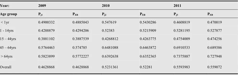
, thereby completely spe-cifying them. In our analyses, we obtain the yearly results for Bayesian Sequential (see Table 1).The result is plotted as shown in Figure 1. Comparing the yearly basis estimated sample proportions and EB proportions as well as va-riances of estimated sample proportions and EB propor-tions.

Table 1. Comparative Analysis of Estimated Sample Proportions and EB Proportions.

Year: 2009 2010 2011

Age group Pj1 PEB Pj2 PEB Pj3 PEB

< 1yr 0.4900332 0.4885043 0.547619 0.5430286 0.4608819 0.470019

1 - 14yrs 0.4288879 0.4294206 0.52383 0.5215909 0.5281195 0.527877

15 – 44yrs 0.3881102 0.3887539 0.4268812 0.4263775 0.4754009 0.474256

45 – 64yrs 0.5764463 0.574785 0.6481088 0.6463872 0.6910533 0.689386

> 64yrs 0.5823899 0.5772227 0.6392638 0.6352365 0.7375887 0.727948

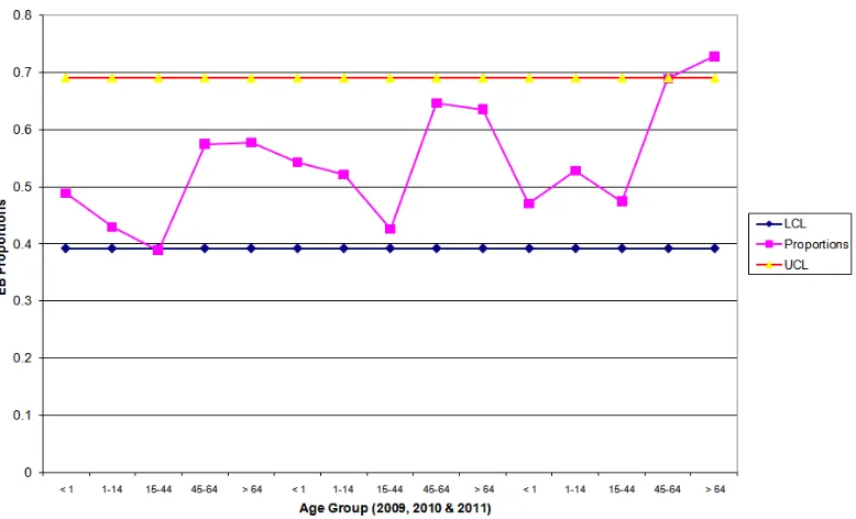
Figure 1.The control chart for Bayesian Sequential of EB proportion.

The result shows that the chart for patients between the ages of 15-44years (0.389) in 2009 is out of control. This implies that among the people that make use of the hospital the age bracket 15 – 44 records very high figure compared to others. In 2011 the result shows that there is a shift in the ages of the patients that attended the hospital from 15-44 years to 44-64 and 64 and above respectively (see Table 1 and Figure 1 above respectively). The result shows that this new approach is able to identify a small or slight shift that

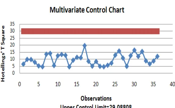
may occur among those that attended the hospital. Table 2 is the estimated values obtained for the covariance’s and Table 3 is the variance and covariance values obtained from computation of Hotellings. Comparing the results of figures 1 and 2, figure 2 cannot identify any slight change that occur while the result of the sequential Bayesian anal-ysis does. Also the values of the variances obtained from the sequential Bayesian analysis are better than that of Ho-tellings.

Table 2. Comparative Analysis of Variances of Estimated Sample Proportions and EB Proportions.

Year: 2009 2010 2011

Age group Var(Pj1) Var(PEB) Var(Pj2) Age group Var(Pj1) Var(PEB)

< 1yr 0.00042 0.00039 0.00037 0.00034 0.00035 0.00031

1 - 14yrs 0.00011 0.00011 0.00011 0.00010 0.00011 0.00011

15 - 44yrs 0.00006 0.00006 0.00006 0.00006 0.00007 0.00007

45 - 64yrs 0.00010 0.00010 0.00010 0.00009 0.00009 0.00009

> 64yrs 0.00031 0.00029 0.00028 0.00027 0.00023 0.00021

Overall 0.00002 0.00002 0.00002 0.00002 0.00003 0.00002

Table 3. Computation of variance of Hotellings’ T Square.

under 1yr 1 - 14YRS 15 - 44YRS 45 - 64YRS 65YRS & ABOVE under 1yr 72.60635 77.31905 182.14286 152.22063 71.78571

1 - 14YRS 77.31905 692.25 652.9 291.04048 150.93571

15 - 44YRS 182.14286 652.9 2473 172.21429 -2.75714

45 - 64YRS 152.22063 291.04048 172.21429 843.97063 393.19286

Figure 2. The control chart for Multivariate HotellingsT24. Conclusion.

This paper has been able to used a Bayesian sequential estimation control chart to determine a small shift that can easily show an out of control signals. Also the phase II approach which involves sequential collection of data over a period of time is adopted in this research using National Orthopaedic data and the result is compared with the con-ventional Hotellings’ T2. Bayesian sequential estimation of proportion is suitable to identify and slight change that occurs than the usual or conventional technique. Similarly, the overall variances of the proportions tend more to zero over the three years under review than that of the variance of Hotellings’ T square. Thus, the results show that the EB estimators are better estimators on the basis of efficiency and consistency properties of good estimators.

References

[1] Resul Oduk (2012) Control Charts for Serially Dependent Multivariate Data Thesis submitted to the Department of In-formatics and Mathematical Modeling at Technical Univer-sity of Denmark in partial fulfillment of the requirements for the degree of Master of Science in Mathematical Model-ing and Computation Technical University Of Denmark. [2] Shewart W.A (1952) The Application of Statistics as an aid

in maintaining quality of a manufactured product” Journal of American Statistical Association: 546-548.

[3] Shewhart WA, (1986), Statistical Method from the View-point of Quality Control General Publishing Company, ISBN 0-486-65232-7.

[4] Shewhart WA, Economic control of quality of manufactured product (1931), Princeton, NJ:Reinhold Co.

[5] Woodall, W. H. (2000). “Controversies and Contradictions in Statistical Process Control” (with discussion). Journal of Quality Technology 32, pp. 341–378. (available at ww.asq.Org/pub/jqt).

[6] Woodall, W.H. Review of Improving Healthcare with Con-trol Charts by Raymond G. Carey, Journal of Quality Tech-nology, 36, 336-338 (2004). 23.

[7] Woodall, W.H. Use of control charts in health-care and pub-lic-health surveillance (with discussion), Journal of Quality Technology, 38, 89-104 (2006).

[8] Lee, P. (2004), Bayesian Statistics An Introduction, Hodder Arnold, New York.

[9] Brandel, J. (2004), Empirical Bayes Methods for missing data analysis, Department of Mathematics Uppsala Univer-sity, Project Report.

[10] Carlin, B. P. and Louis, T. A. (2000b), Bayes and Empirical Bayes Methods for Data Analysis, Boca Raton, Florida: Chapman and Hall/CRC Press.