Parameter Screening and Optimisation for
ILP using Designed Experiments
Ashwin Srinivasan [email protected]
School of Mathematical Sciences & ICT South Asian University
New Delhi 110067, India∗
Ganesh Ramakrishnan [email protected]
Dept. of Computer Science and Engineering Indian Institute of Technology Bombay Mumbai, India
Editor: Luc De Raedt
Abstract
Reports of experiments conducted with an Inductive Logic Programming system rarely describe how specific values of parameters of the system are arrived at when constructing models. Usu-ally, no attempt is made to identify sensitive parameters, and those that are used are often given “factory-supplied” default values, or values obtained from some non-systematic exploratory anal-ysis. The immediate consequence of this is, of course, that it is not clear if better models could have been obtained if some form of parameter selection and optimisation had been performed. Questions follow inevitably on the experiments themselves: specifically, are all algorithms being treated fairly, and is the exploratory phase sufficiently well-defined to allow the experiments to be replicated? In this paper, we investigate the use of parameter selection and optimisation techniques grouped under the study of experimental design. Screening and response surface methods deter-mine, in turn, sensitive parameters and good values for these parameters. Screening is done here by constructing a stepwise regression model relating the utility of an ILP system’s hypothesis to its input parameters, using systematic combinations of values of input parameters (technically speak-ing, we use a two-level fractional factorial design of the input parameters). The parameters used by the regression model are taken to be the sensitive parameters for the system for that application. We then seek an assignment of values to these sensitive parameters that maximise the utility of the ILP model. This is done using the technique of constructing a local “response surface”. The parameters are then changed following the path of steepest ascent until a locally optimal value is reached. This combined use of parameter selection and response surface-driven optimisation has a long history of application in industrial engineering, and its role in ILP is demonstrated using well-known benchmarks. The results suggest that computational overheads from this preliminary phase are not substantial, and that much can be gained, both on improving system performance and on enabling controlled experimentation, by adopting well-established procedures such as the ones proposed here.
Keywords: inductive logic programming, parameter screening and optimisation, experimental design
1. Introduction
We are concerned in this paper with Inductive Logic Programming (ILP) primarily as a tool for constructing models. Specifications of the appropriate use of a tool, its testing, and analysis of benefits and drawbacks over others of a similar nature are matters for the engineer concerned with its routine day-to-day use. Much of the literature on the applications of ILP have, to date, been once-off demonstrations of either the model construction abilities of a specific system, or of the ability of ILP systems to represent and use complex domain-specific relationships (Bratko and Muggleton, 1995; Dzeroski, 2001). It is not surprising, therefore, that there has been little reported on practical issues that arise with the actual use of an ILP system.
Assuming some reasonable solution has been found to difficult practical problems like the ap-propriateness of the representation, choice of relevant “background knowledge”, poor user-interfaces, and efficiency,1 we are concerned here with a substantially simpler issue. Like all model-building methods, an ILP system’s performance is affected by values assigned to input parameters (the term is used here in the sense understood by the computer scientist, and not the statistician). For exam-ple, the model constructed by an ILP system may be affected by the maximal length of clauses, the minimum precision allowed for any clause in the theory, the maximum number of new variables that could appear in any clause, and so. The ILP practitioner is immediately confronted with two questions: (a) Which of these parameters are relevant for the particular application at hand?; and (b) What should their values be in order to get a good model? In an industrial setting, an engineer confronted with similar questions about a complex system—a chemical plant, for example—would try to perform some form of sensitivity analysis to determine an answer to (a), and follow it with an attempt to identify optimal values for the parameters identified. As it stands, experimental applica-tions of ILP usually have not used any such systematic approach. Typically, parameters are given ”factory-supplied” default values, or values obtained from a limited investigation of performance across a few pre-specified values. The immediate consequence of this is that it is not clear if better models could have been obtained if some form of parameter selection and optimisation had been performed. A measure of the unsatisfactory state of affairs is obtained by considering whether it would be acceptable for a chemical engineer to take a similar approach when attempting to identify optimal operating conditions to maximise the yield of his plant.
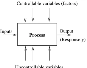
Here take up the questions of screening and optimisation of parameters directly with the only restrictions being that parameter and goodness values are quantitative in nature. The methods we use have origins in optimising industrial processes (Box and Wilson, 1951) and been developed under the broad area concerned with the design and analysis of experiments. This area is concerned principally with discovering something about a black-box system by designing deliberate changes to the system’s input variables, and analysing changes in its output response. The representation of a system is usually as shown in Figure 1(a) (from Montgomery, 2005). The process being modelled transforms some input into an output that is characterised a measurable response y. The system has some controllable factors, and some uncontrollable ones and the goals of an experiment could be to answer questions like: which of the controllable factors are most influential on y; and what levels should these factors be for y to reach an optimal value. The relevance of the setting to the ILP problem we are considering here will be evident in Section 2.
Output
Uncontrollable variables Controllable variables (factors)
Process
(Response y) Inputs
Figure 1: Model of a system used in experimental design (from Montgomery, 2005). The process can be a combination of systems, each modelled by some input-output behaviour.
There are a wide variety of techniques developed within the area of experimental design: we will be concentrating here on some of the simplest, based around the use of regression models. Specifically, using designed variations of input variables, we will use a stepwise linear regression strategy to identify variables most relevant to the ILP system’s output response. This resulting linear model, or response surface, is then used to change progressively the values of the relevant variables until a locally optimal value of the output is reached. We demonstrate this approach empirically on some ILP benchmarks.
The rest of this paper is organised as follows. Section 2 describes a black-box view of ILP systems that we adopt in this paper. Section 3 describes work in ILP and the broader area of Machine Learning related to the goals of this paper. Section 4 describes details of techniques from the field of experimental design that are relevant to the paper. Section 5 describes, first, two empirical studies. The studies demonstrate how, for a given set of inputs, parameter screening and selection using designed experiments yields a better model than simply using default values, or performing an exhaustive combination of pre-determined values for parameters. They also demonstrate how, if inputs are changed, then both the set of relevant parameters and their values can change. These experiments are then followed up with others that use six other well-known benchmark data sets. The results confirm the findings from the primary investigation; and also demonstrate the relevance of this work to the controlled comparisons of ILP systems. Section 6 concludes the paper. The paper is accompanied by two appendices that provide standard material from the literature concerned with the construction of linear models, and with specific aspects of the optimisation method used here.
2. An ILP System as a Black-Box
Bruynooghe, 1992) and more recently, programs that capture complex probabilistic relationships amongst objects (the area of statistical relational learning: see Getoor and Taskar, 2007).
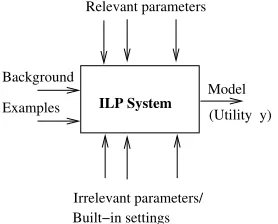
While much effort has been invested in clarifying, in the form of a specification, what constitutes different kinds ILP systems (see, for example Muggleton and Raedt, 1994), in this paper, we take an engineer’s view. In this, an ILP implementation is simply a machine learning (ML) system that, given some inputs—in usual ILP terminology, background knowledge and examples—and settings for parameters, some of which are under the control of the engineer, produces an output model by performing some form of optimisation (see Figure 2). For example, many ILP systems that explore the space of alternatives imposed by the inverse entailment setting proposed in Muggleton (1995) could be seen as performing a form of discrete optimisation, using some approximation to a branch-and-bound search procedure. The task of the system engineer is then to tune the parameters under his or her control to enable the system to return the best performance.2 In Srinivasan (2001b), for example, it is demonstrated how widely varying performance can be obtained by varying a single parameter (the minimum accuracy of clauses found in a search).
Model (Utility y)
ILP System
Irrelevant parameters/ Relevant parameters
Background
Examples
Built−in settings
Figure 2: An system engineer’s view of an ILP system. We are assuming here that “Background” includes syntactic and semantic constraints on acceptable models. “Built-in settings” are the result of decisions made in the design of the ILP system. An example is the optimisation function used by the system.
The immediate difficulty is, of course, that it is usually impractical to examine the system’s performance by enumerating every possible combination of values for the controllable parameters. With ILP systems there are two further difficulties. First, it may often not be known beforehand which parameters are actually relevant to system for the problem being solved. The system Aleph (Srinivasan, 1999) provides perhaps the most clear instance of this: see Figure 3. Second, mod-els constructed, and hence system performance, can vary even if all inputs and parameters have fixed values: for example, the system may use a search strategy that employ some random choices (Zelezny et al., 2002 provides an example of such a strategy).
1. The following parameters can affect the size of the search space: i, clauselength, nodes, minpos, minacc,
noise, explore, best, openlist, splitvars. 2. The following parameters affect the type of search:
search, evalfn, refine, samplesize.
3. The following parameters have an effect on the speed of execution: caching, lazy_negs, proof_strategy, depth,
lazy_on_cost, lazy_on_contradiction, searchtime, prooftime.
4. The following parameters alter the way things are presented to the user: print, record, portray_hypothesis, portray_search,
portray_literals, verbosity,
5. The following parameters are concerned with testing theories: test_pos, test_neg, train_pos, train_neg.
Figure 3: A categorisation of some of the parameters of the ILP system Aleph (reproduced from Srinivasan, 1999). Not all of these are relevant to every problem being solved.
3. Related Work on Parameter Screening and Optimisation
Within ILP, no significant attention has been paid to the problem of parameter screening or optimi-sation. Reports in the literature rarely contain any discussion of sensitive parameters of the system or their values. Of 100 experimental studies reported in papers presented between 1998 and 2008 to the principal conference in the area, none attempt any form of screening for relevant parameters. 17 describe settings for some pre-selected parameters—usually one—from performance estimates obtained during an enumerative search over some small set of possible values (that is, effectively using the wrapper approach of Kohavi and John, 1995). 38 reports, however, mention values as-signed to some parameters, without elucidating how these values were reached (on occasions, these were just the default values provided by the system). The work in Srinivasan (2001b) can be seen as addressing the question of optimal values for several input parameters somewhat indirectly by first constructing an “operating characteristic curve” that describes the performance of an ILP system across a range of values for the relevant parameters. While no method is proposed for identifying the parameters themselves, the characteristic curve provides a way of optimally selecting amongst models, provided model goodness is restricted to a specific class (that of cost functions that are linear in the error-rates). . Since each model is obtained from a particular combination of values for relevant parameters, we are able to identify the values that resulted in the best model for the task. The procedure is somewhat reminiscent of putting the cart before the horse though, requiring us to identify all models on the characteristic curve first.
differentiable function of the parameters (almost) everywhere. While Bengio assumes a training cri-terion that is quadratic in the parameters, Keerthi et al. (2006) present a fast method for computing the gradient of a validation function with respect to parameters for a range of SVM models. Their method only needs a single linear system of equations to be solved. Unfortunately, it is not possible to directly adapt these methods to ILP systems. In almost all ILP settings, the training criterion cannot be even expressed in closed form, let alone being a differentiable and continuous function of the parameters. That is, what can be done at best is to treat the ILP system is a black box (as we have done in the previous section) and empirically observe variations in its response to changes in the values of the parameters.
Methods have been developed that use such empirically observed responses to direct the assign-ment of values to relevant parameters. The seminal work in Kohavi and John (1995) introduced the “wrapper” approach to parameter optimisation, in which responses from a ML system are used to direct a heuristic search through combinations of possible values for the parameters. For tractabil-ity, these values are discretised a priori, and approach essentially performs a sub-optimal search through a finite space of what are called k-level full-factorial designs in this paper (the k refers to the number of discrete values: more on such designs in the next section). In this paper, we use a exhaustive search through such a space as a baseline for comparison against a gradient-based opti-misation method. The results from the exhaustive search clearly represent an upper-bound on the results achievable by any heuristic search through the same space.
The work described in Baz et al. (2007) is concerned with determining parameter values that minimise the computation time of mixed integer linear programming (MILP) systems. As with the ILP systems we consider here, the MILP solvers have many parameters, with no clear relationships known amongst them; and the objective function cannot be expressed as a closed form function of these parameters. Their approach is to select an initial set of values for the hyperparameters using some sampling design. The response of the MILP solver is then obtained, from which a ML system is used to construct a model relating the response to parameter values. This model is then used to suggest new values for some subset of the parameters. For example, if the model used is a regression tree, then the parameters used in the top 2 levels of the tree (the choice of 2 is arbitrary, but no method is proposed for automating this choice) are selected and additional sets of values obtained for the parameters (the exact procedure of how this is done is not elaborated upon). The set that results in the best performance is returned. This work can be seen as a case of exhaustive enumeration of responses in a k-level full factorial design, followed by a single stage of ad hoc non-linear regression-based parameter screening and optimisation.
The problem of screening and tuning of parameters to optimise a system’s performance has been studied extensively in areas of industrial engineering, using results obtained from the design and analysis of experiments. It is our intention in this paper to investigate the application of techniques developed in these areas to ILP, and we summarise some of the relevant ideas next.
4. Design and Analysis of Experiments
by external sources of variation; and (b) Maximise (or minimise) a system’s performance. In turn, these raise questions like the following: which factors are important for the response variables; what values should be given to these factors to maximise (or minimise) the values of the response vari-ables; what values should be give to the factors in order that variability in the response is minimal, and so on.
In this paper, we will restrict ourselves to a single response variable and the analysis of ex-perimental designs by multiple regression. It follows, therefore, that we are restricted in turn to quantitative factors only. Further, by “experimental design” we will mean nothing more than a se-lection of points from the factor-space, in order that a statistically sound relationship between the factors and the response variable can be obtained. Each factor-level combination will constitute an experiment, and a design will therefore require us to specify the experiments and, if necessary, the number of replications of each experiment.
4.1 Screening using Factorial Designs
We first consider designs appropriate for screening. By this, we mean deciding which of a set of potentially relevant factors are really important, statistically speaking. The usual approach adopted is what is termed a 2-level factorial design. In this, each factor is taken to have just two levels (encoded as “-1” and “+1”, say),3and the effect observed on the response variable of changing the levels of each factor. It is evident that with k factors, this will result in 2kexperiments, each of which may need to be repeated in case there is some source of random variation in the response variable. For example, with two factors, conducting a 22full factorial design will result in a table such as the one shown in Figure 4
We are then able to construct a regression model relating the response variable to the factors:
y=b0+b1x1+b2x2+b3x1x2.
The model describes the effect of each factor x1,2and interactive effect x1x2of the two factors on y.4 It is usual also to add “centre points” to the design in the form of experiments that obtain values for y for x1=0 and x2=0. The results of these experiments will not contribute to estimation of the coefficients b1,2,3(since the xiare all 0s), but allows us to obtain a better estimate for the value of b0. Further, it is also the case that with a 2-level full factorial design only linear effects can be estimated (that is, the effect of terms like x2i cannot be obtained: in general, a nthorder polynomial will require n+1 levels for each factor). In this paper, we will use the coefficients of the regression model to guide the screening of parameters: that is, parameters with coefficients significantly different from 0 will be taken to be relevant (more on this in Appendix A).
Clearly, the number of experiments required in a full factorial design constitute a substantial computational burden, especially as the number of factors increase. Consider, however, the role these experiments play in the regression model. Some are necessary for estimating the effects of each factor (that is, the coefficients of x1,x2,x3, . . .: usually called the “main effects”), others for estimating the coefficients for two-way interactions (the coefficients of x1x2, x1x3, . . . ) , others for three-way interactions (x1x2x3, . . . ) and so on. However, in a screening stage, all that we wish to do is to identify the main effects. This can usually be done with fewer than the 2k experiments needed
3. One way to achieve the coded value x of a factor X is as follows. Let X−and X+be the minimum and maximum values of X (these are pre-specified). Then x=X(−X(+X−++X−)X−/)2/2.
Expt. Factor Factor Response
x1 x2 y
E1 -1 -1 . . .
E2 -1 +1 . . .
E3 +1 -1 . . .
E4 +1 +1 . . .
(a)
x1 2
x
−1 +1
−1 +1
(b)
Figure 4: (a) A 2-level full factorial design for two factors; and (b) a graphical representation of the design.
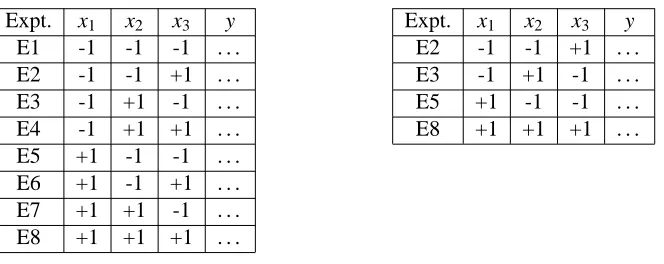
for a full factorial design with k factors. The result is a 2-level “fractional” factorial design. Figure 5 below illustrates a 2-level fractional factorial design for 3 factors that uses half the number of experiments to estimate the main effects (from Steppan et al., 1998).
Expt. x1 x2 x3 y Expt. x1 x2 x3 y
E1 -1 -1 -1 . . . E2 -1 -1 +1 . . .
E2 -1 -1 +1 . . . E3 -1 +1 -1 . . .
E3 -1 +1 -1 . . . E5 +1 -1 -1 . . .
E4 -1 +1 +1 . . . E8 +1 +1 +1 . . .
E5 +1 -1 -1 . . . E6 +1 -1 +1 . . . E7 +1 +1 -1 . . . E8 +1 +1 +1 . . .
Figure 5: A full 2-level factorial design for 3 factors (left) and a “half fraction” design (right).
con-founded with each other. This has some direct implications when constructing regression models using the fractional table. In effect, instead of the full regression model:
y=b0+b1x1+b2x2+b3x3+b4x1x2+b5x1x3+b6x2x3
we are reduced to obtaining the following model:
y=b0+b′1(x1+x2x3) +b′2(x2+x1x3) +b′3(x3+x1x2).
In fact, a regression program will be unable, for example, to distinguish the regression model above from this one:
y=b0+b′′1x1+b′′2x2+b′′3x3 or even this:
y=b0+b′′′1x1+b′′′2x2+b′′′3x1x2.
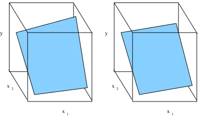
The b′′i and b′′′i will differ from the b′iby a factor of 2, but this will not change the model’s fit of the data, since the corresponding independent variables in the regression equation would be halved (x1 instead of x1+x2x3and so on). Thus, the price for fractional experiments is therefore, that we will in general, be unable to distinguish the effects of all the terms in the full regression model. However, if it is our intention—as it is in the screening stage—only to estimate the main effects (such models are also called “first-order” models), then we can ignore interactions (see Figure 6). Main effects can be estimated with a table that is a fraction required by the full factorial design: for example, the half fraction in Figure 5 is sufficient to obtain a regression equation with just the main effects x1, x2 and x3.5
1 x 2
x y
1 x 2
x y
Figure 6: A surface with a “twist” arising from interactions between the factors (left) and a planar approximation that ignores this twist (right). For the purpose of estimating the main effects, the surface on the right is adequate, as it shows that x2has a much bigger effect than x1on the response y (we are assuming here that x1and x2represent coded values on the same scale).
More details on fractional designs are provided in Appendix B. We use the techniques and results described there to direct the screening of factors by focusing on a linear model that contains the main effects only:
y=b0+b1x1+b2x2+···+bkxk.
Depending on the number of factors, this can be done with a fractional designs of “Resolution III” or above (see Appendix B). Standard tests of significance can be performed on each of the coefficients b1,b2, . . . ,bk to screen factors for relevance (the null and alternative hypotheses in each case are
H0: bi =0 and H1: bi 6=0). In fact, this test is the basis for inclusion or exclusion of factors by
stepwise regression procedures (see Appendix A). Using such a procedure would naturally return a model with only the relevant factors (the use of stepwise regression is also the preferred method for sensitivity analysis suggested at the end of the extensive survey in Helton et al., 2006).
4.2 Optimisation Using the Response Surface
Suppose screening in the manner just described yields a set of k relevant factors from a original set of n factors (which we will denote here as x1,x2, . . . ,xkfor convenience). We are now in the position
of describing the functional relationship between the expected value of the response variable and the relevant factors, by the “response surface”:
E(y) = f(x1,x2, . . . ,xk).
Usually, f is taken to be some low-order polynomial, either a first-order model involving only the main effects x1,x2, . . .(recall that if stepwise regression procedure is used at the screening stage, then this is the model that would be obtained):
y=b0+ k
∑
i=1bixi
or a second-order model involving quadratic terms like x21,x22, . . .and linear interaction terms like x1x2,x1x3, . . .:
y=b0+
k
∑
i=1bixi+ k
∑
i=1biix2i + k
∑
i=1∑
j>ibi jxixj.
Clearly, if first-order models are adequate (this can be checked by an analysis of how well the model fits the data: see Appendix A) then much of the effort expended in the screening stage can be re-used (for example, we can use the model constructed by stepwise regression as the response surface model). A second-order model, on the other hand, will require experiments involving addi-tional levels for each factor, and some effort has been invested in the literature on determining these levels. Since first-order models are all that are used in this paper, we do not pursue this further here, and refer the reader to a standard text like Montgomery (2005) for more details.
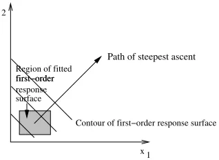
further increase in the response is observed. At this point, a new first-order response surface is constructed, and the process repeated until it is evident that a first-order model is inadequate (or no more increases are possible). If the fit of the first-order model is poor, a more detailed model is then obtained—usually a second-order model, using additional levels for factors—and its stationary point obtained. The basic idea is illustrated in Figure 7 (from Montgomery, 2005).
x x
Path of steepest ascent
Contour of first−order response surface Region of fitted
first−order first−order response surface
1 2
Figure 7: Sequential optimisation of the response surface using the path of steepest ascent. A first-order response surface is obtained in the shaded region. The factors are then changed to move along a direction that gives the maximum increase in the response variable.
Now, we can view the response y to be given by a scalar field f that at each point x1,x2, . . . ,xk
gives the response f(x1,x2, . . . ,xk). Then, from standard vector calculus, the gradient of f at the
point gives the direction in which the response will change most quickly (that is, the direction of steepest ascent: see Appendix B). This gradient, usually denoted∇f , is given by
∂ f ∂x1,
∂f ∂x2, . . . ,
∂f ∂xk
. The sequential optimisation of the response surface just described involves calculating the gradient of the first-order model at the centre, or origin, of the experimental design (x1=x2=···=0). For a model of the form f(x1, . . . ,xk) =b0+b1x1+···+bkxk,∇f is simply(b1, . . . ,bk). For convenience,
let us take b1 to have the largest absolute value. Then, along the direction of∇f , a unit change in x1 will result in a change of b2/b1 units of x2, b3/b1 units of x3 and so on. Sequential response optimisation proceeds by starting at the origin and increasing the xi along ∇f until increases in
the response y is observed. Each such increase results in a new experiment to be performed (see Figure 8, for an example with 3 factors).
4.3 Screening and Optimisation for ILP
We are now in a position to put together the material in the previous sections to state more fully a procedure for screening and optimisation of parameters for an ILP system:
SO: Screen quantitative parameters using a two-level fractional factorial design, and optimise val-ues using the response surface.
ScreenFrac. Screen for relevant parameters using the following steps:
S1. Decide on a set of n quantitative parameters of the ILP system that are of potential relevance. These are the factors xi in the sense just described. Take some
Expt. Factor Factor Factor Response
x1 x2 x3 y
E9 0 0 0 . . .
E10 δ b2
b1δ
b3
b1δ . . .
E11 2δ 2b2
b1 δ
2b3
b1 δ . . .
E12 3δ 3b2
b1 δ
3b3
b1 δ . . .
. . . .
Figure 8: Sequential experiments that obtain new values for y by moving in the direction of the gradient to b0+b1x1+b2x2+b3x3. Experiments E1–E8 are as in Figure 5.
of its predictive accuracy—as the response variable y (we will assume here that we wish to maximise the response).
S2. Decide on on two levels (“low” and “high” values) for each of the factors. These are then coded as±1.
S3. Devise a two-level fractional factorial design of Resolution III or higher, and obtain values of y for each experiment (or replicates of values of y, if so required).
S4. Construct a first-order regression model to estimate the role of the main effects xi
on y. Retain only those factors that are important, by examining the magnitude and significance of the coefficients of the xiin the regression model (alternatively, only
those factors found by a stepwise regression procedure are retained: see Appendix A).
OptimiseRSM. Optimise values of relevant parameters using the following steps:
O1. Construct a first-order response surface using the relevant factors only (this is not needed if stepwise regression was used at the screening stage). If no adequate model is obtained, then return the combination of factor-values that gave the best response at the screening stage. Otherwise go to Step O2.
O2. Progressively obtain new values for y by changing the relevant parameters along the gradient to the response surface. Stop when no increases in y are observed.6 O3. If needed, construct a new first-order response surface. If this surface is adequate,
then return to Step O2. Otherwise, go to Step O4.
O4. If needed, construct a second-order response surface. Return the optimum values of the relevant factors using the second-order surface, or from the last set of values from Step O2.7
6. In practice, this is taken to mean that no increases have been observed for some number of consecutive experimental runs: the so-called “k-in-a-row” stopping rule.
We contrast OptimiseRSM with the multi-level full factorial design below, which has been used on a few occasions within the ILP literature:
OptimiseFact. Optimise values of relevant parameters using the following steps:
O1′. Decide on on multiple levels for each of the relevant factors.
O2′. Devise a full factorial design by combing each of the levels of the factors against those of the others. For each such combination, obtain values of y for each experiment (or replicates of values of y, if so required).
O3′. Select the combination of values that yielded the highest value of y (including those obtained at the screening stage).
This procedure, a multi-level full factorial design, is the basis of the wrapper-based optimisation method in Kohavi and John (1995), recast in the terminology of experimental design. A simplified analysis gives us some feel of the complexity of SO. SO conducts some fraction of 2nexperiments in the ScreenFrac stage, followed by those conducted in OptimiseRSM. Suppose we always conduct a 2n−p-fractional design at the screening stage, and that this stage results in no more than r variables being selected as relevant. Further, let each round of sequential optimisation consist of s experiments in Step O2. Let there be m such rounds of sequential optimisation, each followed by a new first-order model in Step O3 (since there are r variables, building this model will require an additional r+1 experiments). Finally a second-order model is constructed (Step O4), using a central composite design. Then the total number of experiments conducted by SO is: 2n−p(screening) + ms (sequential optimisation) +(m−1)(r+1)(new first-order models) + 2r+1 (second-order model). In the case that only one round of sequential experimentation is performed (that is, m=1) and no additional first- or second-order models are constructed, the number of experiments is simply 2n−p+s. It is evident that a procedure SO′ that employs ScreenFrac followed by OptimiseFact would always perform 2n−p+lrexperiments (assuming, for simplicity, that all relevant factors are taken to have l
levels during the optimisation stage). This is no more than 2n−p+ln. Clarification is needed on the following additional questions:
1. What is to be done if a first-order model cannot be constructed in the screening stage? The usual approach in response-surface methodology is then to examine a second-order response surface. We take the position in this paper that none of the parameters are especially relevant, and simply assign them their default values.
employing a gradient ascent method, we are clearly attempting to minimise the number of experiments by moving along the direction of maximum change. Experimental evidence of overfitting usually also comes to light by increasing the number of data sets on which the procedure is tested (see Section 5.4).
3. What is to be done if the local maximum reached, either by optimising the response-surface or in the multi-level factorial design is not unique? That is, a number of different parameter settings return a maximal value, and we take all of these as being equally likely. The final performance values will thus be the average of the final performance values from each of these settings.
5. Empirical Evaluation
We will first briefly state the aims of the experimental evaluation. Descriptions of the materials and our experimental methodology will follow. We will finally present detailed experimental results.
5.1 Aims
Our aim here is to demonstrate the utility of the screening and optimisation procedure SO that we have described in Section 4.3 (that is, SO is ScreenFrac followed by OptimiseRSM). We assess this utility by comparing the ILP system when it employs SO against the performance of the sys-tem when it uses one of following alternatives: Default, in which no screening or optimisation is performed and default values provided for all parameters are used; and SO′, in which screen-ing is performed as in SO, but a multi-level full factorial design is used for optimisation (that is, SO′is ScreenFrac followed by OptimiseFact). Specifically, we intend to investigate the following conjectures:
C1. Using SO is better than using Default; and
C2. Using SO is better than using SO′.
In both cases, “better” is short-form for stating that an ILP system that uses SO has better final performance; or in the case of ties, requires fewer experiments than the alternative.
5.2 Materials
In this section we explain (i) the two datasets, (ii) the systems for experimental design and ILP and (iii) the hardware employed in our experiments.
5.2.1 DOMAINS
investigate the conjectures C1 and C2 with minimal and maximal amount of background knowledge contained in these benchmarks. That is:
Mutagenesis. We consider background information in the sets M0 and M0–M4, descriptions of which are reproduced below from Srinivasan (2001b):
M0. Molecular description at the atomic level. This includes the atom and bond structure, the partial charges on atoms, and arithmetic constraints (equalities and inequalities). There are 5 predicates in this group;
M1. Structural properties identified by experts as being related to mutagenic activity. These are: the presence of three or more benzene rings, and membership in a class of com-pounds called acenthrylenes. There are 2 predicates in this group;
M2. Chemical properties identified by experts as being related to mutagenic activity, along with arithmetic constraints (equalities and inequalities) The chemical properties are: the energy level of the lowest unoccupied molecular orbital (“LUMO”) in the compound, an artificial property related to this energy level (see Debnath et al., 1991), and the hydrophobicity of the compound. There are 6 predicates in this group;
M3. Generic planar groups. These include generic structures like benzene rings, methyl groups, etc., and predicates to determine connectivity amongst such groups. There are 14 predicates in this group; and
M4. Three-dimensional structure. These include the positions of individual atoms, and con-straints on distances between atom-pairs. There are 2 predicates in this group.
Carcinogenesis. We consider background information in the sets C0 and C0–C3, descriptions of which reproduced below, once again from Srinivasan (2001b):
C0. Molecular description at the atomic level. This is similar to M0 above and is comprised of 5 predicates;
C1. Toxicity properties identified by experts as being related to carcinogenic activity, and arithmetic constraints. These are an interpretation of the descriptions in Ashby and Tennant (1991), and are contained within the definitions of 5 predicates;
C2. Short-term assays for genetic risks. These include the Salmonella assay, in-vivo tests for the induction of micro-nuclei in rat and mouse bone marrow etc. The test results are simply “positive” or “negative” depending on the response and are encoded by a single predicate definition; and
C3. Generic planar groups. These are similar to M3 above, extended to 30 predicate defini-tions.
We will henceforth refer to background knowledge with the definitions in M0 (respectively, C0) as Bminand with the definitions in M0–M4 (respectively, C0–C3) as Bmax.
5.2.2 ALGORITHMS ANDMACHINES
5.3 Method
Our method for the preliminary experiments is straightforward:
For each problem (Mutagenesis and Carcinogenesis) and each level of background knowledge (Bminand Bmax):
1. Construct a model with the ILP system using default values for all parameters of the ILP system. Call this model ILP+Default.
2. Select a set of n quantitative parameters of the ILP system as being potentially relevant. Use the procedure ScreenFrac described in Section 4.3 to screen this set using a frac-tional factorial design of Resolution III or higher. Let this result in a set of relevant variables R.
3. Use the procedure OptimiseRSM in Section 4.3 to obtain values for variables in R. All other parameters of the ILP system are left at their default values. Construct a model using the ILP system with this set of values. Call this model ILP+SO.
4. Decide on l levels for each variable in R and use the procedure OptimiseFact in Section 4.3 to obtain values for the variables in R. All other parameters of the ILP system are left at their default values. Construct a model using the ILP system with this set of values. Call this model ILP+SO′.
5. Compare the performance of the ILP system when it produces as output each of ILP+Default, ILP+SO, and ILP+SO′(see the details below).
We follow the preliminary experiments with experiments on additional data sets and with an additional ILP system. The following details concerning the preliminary experiments are relevant:
1. Since the tasks considered here are binary classification tasks, the performance of the ILP sys-tem in all experiments will be taken to be the classification accuracy of the model produced by the system. By this we mean the usual measure computed from a 2×2 cross-tabulation of actual and predicted classes of instances. We would like the final performance measure to be as unbiased as possible by the experimental estimates obtained during optimisation. One way is to use a technique of “double” or nested cross-validation. That is, the final per-formance value is obtained using k-fold cross-validation (the “outer” cross-validation) and experimental performance values during optimisation is the average of a further (“inner”) k-fold cross-validation using each of the training data sets from the outer cross-validation. This procedure is computationally expensive. We adopt a simpler alternative: we use a 10-fold cross-validation estimate for the final estimate; and for the experimental estimates we use the average of holdout (“validation” set) estimates on each of the training data sets from the outer cross-validation. Thus, the test data in each of the outer cross-validation folds are not available to the ILP system when performing parameter optimisation.
search conducted by the ILP system; Minacc, the minimum accuracy required of any accept-able clause; and Minpos, the minimum number of positive examples to be entailed by any acceptable clause. C and Nodes are directly concerned with the search space explored by the ILP system. Minacc and Minpos are concerned with the quality of results returned (they are equivalent to “precision” and “support” used in the data mining literature). We propose to examine a two-level fractional factorial design, using the levels shown below (the column “Default” refers to the default values for the factors assigned by the Aleph system, and±1 refers to the coded values of the factors):
Factor Levels
Default Low (−1) High (+1)
C 4 4 8
Nodes 5000 5000 10000 Minacc +1 0.75 0.90
Minpos 1 5 10
3. We use a Resolution IV design, that comprises of a randomised presentation of the following 8 experiments (recall the full factorial design will require 24=16 experiments):
Expt. C Nodes Minacc Minpos Accuracy
E1 −1 −1 −1 −1 . . .
E2 −1 −1 +1 +1 . . .
E3 −1 +1 −1 +1 . . .
E4 −1 +1 +1 −1 . . .
E5 +1 −1 −1 +1 . . .
E6 +1 −1 +1 −1 . . .
E7 +1 +1 −1 −1 . . .
E8 +1 +1 +1 +1 . . .
This design was obtained using the software tools for experimental design provided with Step-pan et al. (1998). The “Accuracy” column is the experimental performance obtained for each task, and for each of the two sets of background knowledge in order to screen the four vari-ables for relevance. Additional experiments, and corresponding experimental performance values, will be needed in Step 3 to obtain values of the relevant parameters using the response surface. We restrict ourselves to constructing just one first-order regression model for screen-ing, using the stepwise regression procedure provided by the authors of Steppan et al. (1998). This model is taken to approximate the local response surface: we then proceed to change levels of factors along the normal to this surface in the manner described in Figure 8. Ex-periments are stopped once a maximal value for the response variable is followed by three consecutive runs that yield responses that are no higher.
Composite” (or CC) design (Montgomery, 2005), we will take the (coded) levels to be 0,±1, and±√2.
5. Comparisons of models will be done on the basis of their final performance estimates (see (1) above) (parameter values are obtained from the experimental estimates). In the event of ties, then the model requiring fewer experiments will be preferred. That is, a model is repre-sented by the pair(A,E)(denoting estimated accuracy and number of experiments required to identify the model). Comparisons are then based on the usual definition of a lexicographic ordering on such tuples.
Further, since it is of particular relevance to ILP practitioners, we also test for statistical dif-ferences between the accuracies of ILP+SO and ILP+ Default using results on six additional data sets used in the ILP literature, and separately, by using two different ILP systems. The relevant statistical test is the Wilcoxon signed-rank test (Siegel, 1956). This is a non-parametric test of the null hypothesis that there is no significant difference between the median performance of a pair of algorithms. The test works by ranking the absolute value of the differences observed in perfor-mance of the pair of algorithms. Ties are discarded and the ranks are then given signs depending on whether the performance of the first algorithm is higher or lower than that of the second. If the null hypothesis holds, the sum of the signed ranks should be approximately 0. The probabilities of observing the actual signed rank sum can be obtained by an exact calculation (if the number of entries is less than 10), or by using a normal approximation. We note that the comparing a pair of algorithms using the Wilcoxon test is equivalent to determining if the area under the ROC curves of the algorithms differ significantly (Hand, 1997).
5.4 Results and Discussion
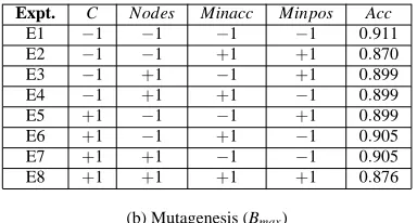
We present first the results concerned with screening for relevant factors. Figure 9 show responses from the ILP system for the preliminary experiments conducted for screening using the fractional design described under “Methods”. The sequence of experiments following this stage for optimising relevant parameter values using: (a) the response surface; and (b) a multi-level full factorial design are in Figures 10 and 11. Finally, a comparison of the three procedures ILP+Default, ILP+SO, and ILP+SO′is in Figure 12. It is this last tabulation that is of direct relevance to the experimental aims of this paper, and we note the following: (1) Although no experimentation is needed for the use of default values, the model obtained with ILP+Default usually has the lowest predictive accuracies (the exception is Carcinogenesis, with Bmin);8 (2) The classification accuracy of ILP+SO is never
lower than that of any of the other methods; (3) When the classification accuracies of ILP+SO and ILP+SO′are comparable, the number of experiments needed by the former is lower.
Taken together, these observations provide prima facie evidence for the conjectures made at the outset of this section, namely:
C1. Using SO is better than using Default; and
C2. Using SO is better than using SO′.
8. We recall that no adequate first-order regression model was obtained for Carcinogenesis (Bmin), resulting in default
Expt. C Nodes Minacc Minpos Acc Expt. C Nodes Minacc Minpos Acc
E1 −1 −1 −1 −1 0.793 E1 −1 −1 −1 −1 0.911
E2 −1 −1 +1 +1 0.644 E2 −1 −1 +1 +1 0.870
E3 −1 +1 −1 +1 0.763 E3 −1 +1 −1 +1 0.899
E4 −1 +1 +1 −1 0.669 E4 −1 +1 +1 −1 0.899
E5 +1 −1 −1 +1 0.757 E5 +1 −1 −1 +1 0.899
E6 +1 −1 +1 −1 0.728 E6 +1 −1 +1 −1 0.905
E7 +1 +1 −1 −1 0.787 E7 +1 +1 −1 −1 0.905
E8 +1 +1 +1 +1 0.669 E8 +1 +1 +1 +1 0.876
(a) Mutagenesis (Bmin) (b) Mutagenesis (Bmax)
Acc=0.726−0.049 Minacc−0.018 Minpos Acc=0.896−0.009 Minpos−0.008 Minacc
Expt. C Nodes Minacc Minpos Acc Expt. C Nodes Minacc Minpos Acc
E1 −1 −1 −1 −1 0.464 E1 −1 −1 −1 −1 0.572
E2 −1 −1 +1 +1 0.461 E2 −1 −1 +1 +1 0.595
E3 −1 +1 −1 +1 0.444 E3 −1 +1 −1 +1 0.507
E4 −1 +1 +1 −1 0.447 E4 −1 +1 +1 −1 0.576
E5 +1 −1 −1 +1 0.457 E5 +1 −1 −1 +1 0.585
E6 +1 −1 +1 −1 0.451 E6 +1 −1 +1 −1 0.526
E7 +1 +1 −1 −1 0.467 E7 +1 +1 −1 −1 0.523
E8 +1 +1 +1 +1 0.461 E8 +1 +1 +1 +1 0.546
(c) Carcinogenesis (Bmin) (d) Carcinogenesis (Bmax) No adequate model Acc=0.554−0.028 Minacc
Figure 9: Screening results (procedure ScreenFrac in Section 4.3). Acc refers to the estimated accuracy of the model. The regression model is built using the “Autofit” option provided in Steppan et al. (1998). This essentially implements the stepwise regression procedure described in Appendix A. Acc refers to the experimental (validation-set) performance of the ILP system. Note that no adequate model is obtained in (c), meaning that the coefficients of all variables have values that are statistically insignificant. In this case, no further optimisation is performed, and all parameters are left at their default values.
We now turn to some broader implications of these results, enumerated in order of seriousness to current ILP practice:
1. The results suggest that default levels for factors need not yield optimal models for all prob-lems, or even when the same problem is given different inputs (here, different background knowledge). This means that using ILP systems just based on default values for parameters— the accepted practice at present—can give misleading estimates of the best response possible from the system. This is illustrated in Figure 13, which shows estimated accuracies on other data sets reported in the literature that also use the Aleph system with default values for all parameters (these data sets have been used widely: see, for example, Landwehr et al., 2006 and Muggleton et al., 2008). Taken with our previous results for the mutagenesis and carcino-genesis data (we will only use the Bmaxresults, as these are the results used in the literature),
Expt. Coded Values Natural Values Acc Expt. Coded Values Natural Values Acc Minacc Minpos Minacc Minpos Minpos Minacc Minpos Minacc
E9 0 0 0.83 8 0.769 E9 0 0 8 0.83 0.899
E10 −0.50 −0.18 0.79 7 0.793 E10 −0.50 −0.42 7 0.79 0.899 E11 −1 −0.36 0.75 7 0.781 E11 −1.0 −0.84 5 0.76 0.911 E12 −1.50 −0.54 0.71 6 0.781 E12 −1.50 −1.26 4 0.73 0.899 E13 −2.00 −0.72 0.67 6 0.692 E13 −2.00 −1.68 3 0.70 0.893 E14 −2.50 −2.10 2 0.67 0.751 (a) Mutagenesis (Bmin) (b) Mutagenesis (Bmax)
Expt. Coded Value Natural Value Acc Minacc Minacc
E9 0 0.83 0.553
E10 −0.50 0.79 0.572
E11 −1 0.75 0.595
E12 −1.50 0.71 0.582 E13 −2.00 0.67 0.592 E14 −2.50 0.63 0.598 E15 −3.00 0.60 0.605 E16 −3.50 0.56 0.609 E17 −4.00 0.52 0.539 E18 −4.50 0.49 0.539 E19 −3.50 0.45 0.539
(c) Carcinogenesis (Bmax)
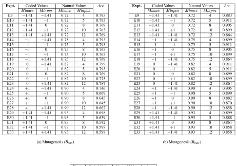
Figure 10: Optimisation using the response surface (procedure OptimiseRSM in Section 4.3). In each case, the response surface used is the first-order regression model found by step-wise regression at the screening stage (shown in Figure 9). Parameters are varied along the path of steepest ascent of experimental performance values for the response variable. Experiments are stopped once a maximal value for the response variable is followed by three consecutive runs that yield responses that are no higher. No optimisation is per-formed for Carcinogenesis (Bmin) since no adequate first-order response surface was
found.
Expt. Coded Values Natural Values Acc Expt. Coded Values Natural Values Acc Minacc Minpos Minacc Minpos Minacc Minpos Minacc Minpos
E9 −1.41 −1.41 0.72 4 0.793 E9 −1.41 −1.41 0.72 4 0.883 E10 −1.41 −1 0.72 5 0.793 E10 −1.41 −1 0.72 5 0.911
E11 −1.41 0 0.72 8 0.769 E11 −1.41 0 0.72 8 0.905
E12 −1.41 +1 0.72 10 0.763 E12 −1.41 +1 0.72 10 0.899 E13 −1.41 +1.41 0.72 12 0.769 E13 −1.41 +1.41 0.72 12 0.864 E14 −1 −1.41 0.75 4 0.793 E14 −1 −1.41 0.75 4 0.899
E15 −1 −1 0.75 5 0.793 E15 −1 −1 0.75 5 0.911
E16 −1 0 0.75 8 0.763 E16 −1 0 0.75 8 0.905
E17 −1 +1 0.75 10 0.763 E17 −1 +1 0.75 10 0.899
E18 −1 +1.41 0.75 12 0.769 E18 −1 +1.41 0.75 12 0.864
E19 0 −1.41 0.82 4 0.799 E19 0 −1.41 0.82 4 0.911
E20 0 −1 0.82 5 0.793 E20 0 −1 0.82 5 0.911
E21 0 0 0.82 8 0.769 E21 0 0 0.82 8 0.899
E22 0 +1 0.82 10 0.775 E22 0 +1 0.82 10 0.899
E23 0 +1.41 0.82 12 0.787 E23 0 +1.41 0.82 12 0.864 E24 +1 −1.41 0.90 4 0.746 E24 +1 −1.41 0.90 4 0.905
E25 +1 −1 0.90 5 0.669 E25 +1 −1 0.90 5 0.899
E26 +1 0 0.90 8 0.645 E26 +1 0 0.90 8 0.882
E27 +1 +1 0.90 10 0.645 E27 +1 +1 0.90 10 0.870
E28 +1 +1.41 0.90 12 0.662 E28 +1 +1.41 0.90 12 0.858 E29 +1.41 −1.41 0.93 4 0.698 E29 +1.41 −1.41 0.93 4 0.899 E30 +1.41 −1 0.93 5 0.639 E30 +1.41 −1 0.93 5 0.888
E31 +1.41 0 0.93 8 0.592 E31 +1.41 0 0.93 8 0.864
E32 +1.41 +1 0.93 10 0.598 E32 +1.41 +1 0.93 10 0.858 E33 +1.41 +1.41 0.93 12 0.598 E33 +1.41 +1.41 0.93 12 0.858
(a) Mutagenesis (Bmin) (b) Mutagenesis (Bmax)
Expt. Coded Value Natural Value Acc Minacc Minacc
E9 −1.41 0.72 0.586
E10 −1 0.75 0.595
E11 0 0.83 0.553
E12 +1 0.90 0.516
E13 +1.41 0.93 0.526 (c) Carcinogenesis (Bmax)
Procedure (Accuracy,Expts.)
Mutagenesis Carcinogenesis
Bmin Bmax Bmin Bmax
ILP+Default (0.755±0.031,0) (0.846±0.026,0) (0.510±0.028,0) (0.504±0.028,0)
ILP+SO (0.803±0.029,13) (0.883±0.023,14) (0.510±0.028,8) (0.591±0.027,19)
ILP+SO′ (0.787±0.030,33) (0.883±0.023,33) (0.510±0.028,8) (0.579±0.027,13)
Figure 12: Comparison of procedures, based on their final performance, using the parameter val-ues obtained from optimising experimental performance. The entries shown are 10-fold cross-validation estimates and the number of experiments needed to obtain the opti-mised value. There is no unbiased estimator of variance for the cross-validation esti-mates (Bengio and Grandvalet, 2004): the standard error reported is computed using the approximation in Breiman et al. (1984).
2. The screening results suggest that as inputs change, so can the relevance of factors (for exam-ple, when the background changes from Bminto Bmaxin Carcinogenesis, Minacc becomes a a
relevant factor). Further evidence for this comes from the “DSSTox” data set (see Figure 15). This means that a once-off choice of relevant factors across all possible inputs can lead to sub-optimal performances from the system for some inputs.
3. Screening, as proposed here, still requires identification of an initial set of variables as factors to be varied (here, these were C, Nodes, Minacc and Minpos). While the set can have any number of elements (all quantitative of course, for the techniques here to be applicable), the choice of these elements remains in the hands of the practitioner using the ILP system. Some element of human expertise of this kind appears unavoidable (and indeed, is even desirable, to prevent pointless experimentation). Additional assistance in the form of including, with each ILP system, a set of potentially sensitive parameters, could be a great help.
4. Optimisation, as proposed here, requires the selection of an appropriate step-size and spec-ification of a stopping criterion for a sequential search conducted along the gradient to the response surface. We have followed the prevalent practice in the field, namely, obtaining the step-size by a process of a binary search over the interval [0,1]; and using a “k-in-a-row” stopping rule (that is, stopping the search if k steps yield no improvement in response). Other techniques exist, and are described in Appendix B.
5. Even if a set of relevant factors are available for a given input, a multi-level full factorial design can be an expensive method to determine appropriate levels. Once done, performance may still be sub-optimal. The results here suggests that experimental studies that ad hoc discretisation followed by exhaustive combinations of the different discrete levels of relevant parameters may not yield the best results.
Data ILP+Default ILP+SO
Mut(42) 0.857±0.054 0.857±0.054 Alz (Amine) 0.714±0.017 0.802±0.015 Alz (Tox) 0.792±0.014 0.872±0.011 Alz (Acetyl) 0.527±0.014 0.774±0.011 Alz (Memory) 0.551±0.020 0.674±0.019 DSSTox 0.647±0.020 0.731±0.018
Figure 13: Estimated accuracies for the Aleph system from some additional data sets used in the literature (Muggleton et al., 2008; Landwehr et al., 2006). The data sets are used in comparative experiments (“System X versus Aleph”) that use default settings for all parameters of Aleph. Accuracy estimates for such models are in the column headed “ILP+Default” (although these exact values do not concern us here, we note that dif-ferences, if any, to accuracies reported in the literature can be attributed to differences in the cross-validation splits used). The column headed “ILP+SO” are final perfor-mance estimates obtained using Aleph with the SO procedure described in the paper, and the method used in the preliminary experiments. Standard errors are calculated as before. The DSSTox background information differ slightly in Muggleton et al. (2008) and Landwehr et al. (2006) and the models here use the variant from Muggleton et al. (2008).
Data ILP+Default ILP+SO ∆ Signed Rank Carcin 0.504 0.591 0.089 +4 Mut (188) 0.846 0.883 0.037 +1
Mut(42) 0.857 0.857 0 –
Alz (Amine) 0.714 0.802 0.088 +5 Alz (Tox) 0.792 0.872 0.080 +2 Alz (Acetyl) 0.527 0.774 0.247 +7 Alz (Memory) 0.551 0.674 0.123 +6 DSSTox 0.647 0.731 0.084 +3
Figure 14: Absolute differences in accuracy∆between the procedures ILP+SO and ILP+Default, and their signed ranks (eliminating ties). The Wilcoxon probability of obtserving the signed ranks under the null hypothesis that median differences are 0, is 0.02 (0.01 for a directional test).
Data ILP+Default ILP + SO
DSSTox (Muggleton et al., 2008) 0.647±0.020 0.731±0.018 DSSTox (Landwehr et al., 2006) 0.631±0.020 0.631±0.020
Data Toplog+Default Toplog+SO ∆ Signed Rank Carcin 0.641 0.623 0.018 −2 Mut (188) 0.840 0.867 0.027 +3.5
Mut(42) 0.881 0.881 0 –
Alz (Amine) 0.704 0.704 0 –
Alz (Tox) 0.672 0.699 0.027 +3.5 Alz (Acetyl) 0.640 0.635 0.005 −1 Alz (Memory) 0.526 0.653 0.127 +5
DSSTox 0.618 0.618 0 –
Figure 16: Absolute differences in accuracy ∆ between the procedures Toplog+SO and Toplog+Default, and their signed ranks (eliminating ties). Once again, we differences, if any, to accuracies reported in the literature can be attributed to differences in the cross-validation splits used. Although the sum of the signed ranks (+9) is in favour of Toplog+SO, the evidence is not statistically significant (that is p>0.05)
ILP studies, but whose value is self-evident. Of course, screening and optimisation experiments would have to be conducted for each system in turn, since the factors relevant to one system (and its levels) would typically have no relation to those of any of the others. We illustrate this in Figures 16–17. The former shows results of applying the procedure SO to a recently proposed ILP system (Toplog) on the data sets we have considered thus far. Parameter screening and op-timisation proceeds for a different set of parameters to those used for Aleph: we have used the parameters Max literals in hypothesis (equivalent to the parameter C in the Aleph experiments), Max singletons in hypothesis, Example in f lation, and Minpos (which has the same meaning as Minpos in the Aleph experiments). The choice of these parameters was based on their use in data files provided with the Toplog program. It is evident from Figure 16 that there is an improve-ment in performance after using SO (the overall sum of signed ranks is in favour of Toplog+SO) although the differences are not statistically significant. This statistical caveat notwithstanding, Fig-ure 17 shows the perils of not comparing like-with-like. FigFig-ure 17(a) shows that having subject both Toplog and Aleph to the same procedure for screening and optimisation (that is, SO), we find no significant difference in their performance. On the other hand, Figure 17(b) shows that performing screening and optimisation on one (Aleph), but not the other (Toplog), can lead to misleading results (that the performance of Aleph is significantly better than Toplog).
6. Concluding Remarks
Data Toplog+SO Aleph+SO ∆ Signed Rank Carcin 0.623 0.591 0.032 −4 Mut (188) 0.867 0.883 0.016 +1 Mut(42) 0.881 0.857 0.024 −3 Alz (Amine) 0.704 0.802 0.070 +5 Alz (Tox) 0.699 0.872 0.173 +8 Alz (Acetyl) 0.635 0.774 0.139 +7 Alz (Memory) 0.653 0.674 0.021 +2 DSSTox 0.618 0.731 0.113 +6
(a)
Data Toplog+Default Aleph+SO ∆ Signed Rank Carcin 0.641 0.591 0.050 −3 Mut (188) 0.840 0.883 0.043 +2 Mut(42) 0.881 0.857 0.024 −1 Alz (Amine) 0.704 0.802 0.098 +4 Alz (Tox) 0.672 0.872 0.200 +8 Alz (Acetyl) 0.640 0.774 0.134 +6 Alz (Memory) 0.526 0.674 0.148 +7 DSSTox 0.618 0.731 0.113 +5
(b)
Figure 17: (a) Absolute differences in accuracy ∆ between the procedures Aleph+SO and Toplog+SO, and their signed ranks (eliminating ties). Although the sum of the signed ranks is in favour of Aleph+SO (+22), the evidence is not statistically significant (that is p>0.05). (b) Absolute differences in accuracy∆between the procedures Aleph+SO and Toplog+Default, and their signed ranks (eliminating ties). The sum of the signed ranks is in favour of Aleph+SO (+28), is now statistically significant (p=0.05 for a non-directional test, p=0.025 for a directional test). Performing the comparison (b) instead of (a) can result in the misleading conclusion that the Aleph system performs significantly better than Toplog on these data sets.
to develop better models with ILP systems. To the best of our knowledge, this is the first time9any such formal framework has been employed for this purpose in ILP.
There are a number of ways in which the work here can be extended further. On the conceptual front, we have concentrated on the simplest forms of designed experiments (sometimes called “clas-sical” DOE). Substantial effort has been expended in developing designs other than the fractional factorial designs used here. Response surface optimisation could also involve more complex mod-els than the simple first-order modmod-els used here. Both options could yield better results than those obtained here. On the experimental front, our emphasis has been on a controlled study of fractional-factorial screening and response-surface optimisation, using well-studied ILP benchmarks. There are clearly many other data sets studied within ILP that could benefit from utilising the techniques proposed. We have also modelled system performance by its estimated accuracy: clearly other measures may be of interest (for example, some combination of the accuracy and complexity of models, in the MDL sense). Finally, it is evident from our results in Figure 17 that there are wider implications of the results here to the work on the comparative study of ILP systems, and to the development of ILP systems as tools for data analysis. Indeed, nothing restricts the procedures here just to ILP, and the same comments apply to many other machine learning systems. Although outside the scope of this paper, these directions are clearly of some importance, and worth pursuing.
Acknowledgments
The authors would like to thank Ravi Kothari of IBM Research—India, for initiating interest in the area of design and analysis of experiments. For much of this work, A.S. was supported by a Ramanujan Fellowship, Dept. of Science and Technology, Government of India; and was at the Dept. of Biotechnology’s Centre of Excellence at the School of Information Technology, Jawaharlal Nehru University, New Delhi.
Appendix A. A Note on Linear Regression Models
In this section we provide details of regression models that are of relevance to this paper. All these details can be obtained in any textbook on statistical modelling: we reproduce them here simply for completeness.
Given a response variable y and variables x1,x2, . . . ,xk, a regression model expresses a
relation-ship between y and the xi as follows:
y= f(x1,x2, . . . ,xk) +ε
where f denotes a systematic functional relationship between y and the xi, and εdenotes random
variation in y that is unrelated to the xi (usually called the error). Usually f is specified as some
mathematical function (for example, a polynomial in the xi) andεby a probability density function
(PDF). The PDF forεis taken to have mean 0 and standard deviationσ: normally the distribution is also taken to be Gaussian. Thus, in a slightly lop-sided way, for a given set of values for the xi, it is easier to think of a random value being chosen for εand then constant f(x1, . . . ,xk) being
added to give the final value of y. From this is evident that y will have a PDF with mean given by E(y) =E(f(x1, . . . ,xk) +ε) = f(x1, . . . ,xk) +E(ε) = f(x1, . . . ,xk)); and standard deviationσ. Thus,
the regression function effectively specifies the expected, or mean value, of y, given the xi. “Linear
regression” refers to the case when the functional relationship is a linear equation of the form:
f(x1, . . . ,xk) =β0+β1x1+···+βkxk.
Here, “linear” refers to being linear in the coefficientsβi. So, the following is also a case of linear
regression:
f(x1, . . . ,xk) =β0+β1x1+···+βkxk+βk+1x21+···+β2kx2k+β2k+1x1x2+···.
To differentiate between these kinds of equation, we denote the former kind which only contain terms x1,x2, . . .as first-order function; and equations of the latter kind which contain quadratic and interaction terms as a second-order function.
In general, assuming we knew the form of f (for example, that it was a first-order function, with errors following a Gaussian distribution with zero mean and varianceσ2), and which of the xi were functionally related to y, we still need to be able to obtain values of theβi from a set of
observations, or data points, giving values for the relevant xi and the corresponding values of y.
Actually, the best we are able to do is obtain estimates ofβi, which we will denote here as bi, along
with some statistical statement on these estimates. The result is a regression model:
ˆ
y=b0+b1x1+b2x2+···.
Thus, with each data point k, we have an associated “residual” given by difference between the value yk for that data point, and the value ˆyk obtained from the regression model. The usual approach for
obtaining the estimates bi is the method of least squares, that attempts to minimise the sum of
squares of the residuals. The details can be found in any standard statistical textbook (for example, Walpole and Myers, 1978).
We now turn to the first of our assumptions, namely, that of the form of the function. The validity of this assumption can be tested by examining how well the model fits the observed data; and, if used for prediction, estimating how well it will predict response values on new data. The degree of model fit is obtained by examining the residuals and calculating first the statistical significance of model. This tests the null hypothesis H0 : b0 =b1 =···=bk =0 (that is, there is no linear
relationship between y and any of the xi). Specifically, the quantity:
F= SSR/k
SSE/(N−1−k)
is calculated, where where SSE refers to the sum of squared residuals (∑Nk=1(yk−yˆk))2, N being
the number of data points); and SSR is the sum of squares of deviations of the model’s response from the mean response (∑Nk=1(yˆ−y))2). F is known to follow the F-distribution with k,N−1−k degrees of freedom (Walpole and Myers, 1978). So, the hypothesis H0can be rejected at some level of significanceα, if the F-value obtained is greater than the value tabulated for Fα,k,N−1−k.