Visualizing Data using t-SNE

Visualizing Data using t-SNE

Laurens van der Maaten [email protected]

TiCC

Tilburg University

P.O. Box 90153, 5000 LE Tilburg, The Netherlands

Geoffrey Hinton [email protected]

Department of Computer Science University of Toronto

6 King’s College Road, M5S 3G4 Toronto, ON, Canada

Editor: Yoshua Bengio

Abstract

We present a new technique called “t-SNE” that visualizes high-dimensional data by giving each datapoint a location in a two or three-dimensional map. The technique is a variation of Stochastic Neighbor Embedding (Hinton and Roweis, 2002) that is much easier to optimize, and produces significantly better visualizations by reducing the tendency to crowd points together in the center of the map. t-SNE is better than existing techniques at creating a single map that reveals structure at many different scales. This is particularly important for high-dimensional data that lie on several different, but related, low-dimensional manifolds, such as images of objects from multiple classes seen from multiple viewpoints. For visualizing the structure of very large data sets, we show how t-SNE can use random walks on neighborhood graphs to allow the implicit structure of all of the data to influence the way in which a subset of the data is displayed. We illustrate the performance of t-SNE on a wide variety of data sets and compare it with many other non-parametric visualization techniques, including Sammon mapping, Isomap, and Locally Linear Embedding. The visualiza-tions produced by t-SNE are significantly better than those produced by the other techniques on almost all of the data sets.

Keywords: visualization, dimensionality reduction, manifold learning, embedding algorithms,

multidimensional scaling

1. Introduction

data to the human observer. This severely limits the applicability of these techniques to real-world data sets that contain thousands of high-dimensional datapoints.

In contrast to the visualization techniques discussed above, dimensionality reduction methods convert the high-dimensional data set

X

Y

{y1,y2, ...,yn}that can be displayed in a scatterplot. In the paper, we refer to the low-dimensional

data representation

Y

da-tapoints as map points. The aim of dimensionality reduction is to preserve as much of the sig-nificant structure of the high-dimensional data as possible in the low-dimensional map. Various techniques for this problem have been proposed that differ in the type of structure they preserve. Traditional dimensionality reduction techniques such as Principal Components Analysis (PCA; Hotelling, 1933) and classical multidimensional scaling (MDS; Torgerson, 1952) are linear tech-niques that focus on keeping the low-dimensional representations of dissimilar datapoints far apart. For high-dimensional data that lies on or near a low-dimensional, non-linear manifold it is usu-ally more important to keep the low-dimensional representations of very similar datapoints close together, which is typically not possible with a linear mapping.

A large number of nonlinear dimensionality reduction techniques that aim to preserve the local structure of data have been proposed, many of which are reviewed by Lee and Verleysen (2007). In particular, we mention the following seven techniques: (1) Sammon mapping (Sammon, 1969), (2) curvilinear components analysis (CCA; Demartines and H´erault, 1997), (3) Stochastic Neighbor Embedding (SNE; Hinton and Roweis, 2002), (4) Isomap (Tenenbaum et al., 2000), (5) Maximum Variance Unfolding (MVU; Weinberger et al., 2004), (6) Locally Linear Embedding (LLE; Roweis and Saul, 2000), and (7) Laplacian Eigenmaps (Belkin and Niyogi, 2002). Despite the strong per-formance of these techniques on artificial data sets, they are often not very successful at visualizing real, high-dimensional data. In particular, most of the techniques are not capable of retaining both the local and the global structure of the data in a single map. For instance, a recent study reveals that even a semi-supervised variant of MVU is not capable of separating handwritten digits into their natural clusters (Song et al., 2007).

In this paper, we describe a way of converting a high-dimensional data set into a matrix of pair-wise similarities and we introduce a new technique, called “t-SNE”, for visualizing the resulting similarity data. t-SNE is capable of capturing much of the local structure of the high-dimensional data very well, while also revealing global structure such as the presence of clusters at several scales. We illustrate the performance of t-SNE by comparing it to the seven dimensionality reduction tech-niques mentioned above on five data sets from a variety of domains. Because of space limitations, most of the(7+1)_×5=40 maps are presented in the supplemental material, but the maps that we present in the paper are sufficient to demonstrate the superiority of t-SNE.

2. Stochastic Neighbor Embedding

Stochastic Neighbor Embedding (SNE) starts by converting the high-dimensional Euclidean dis-tances between datapoints into conditional probabilities that represent similarities.1 The similarity of datapoint xjto datapoint xiis the conditional probability, pj|i, that xiwould pick xjas its neighbor

if neighbors were picked in proportion to their probability density under a Gaussian centered at xi.

For nearby datapoints, pj|i is relatively high, whereas for widely separated datapoints, pj|i will be

almost infinitesimal (for reasonable values of the variance of the Gaussian,σi). Mathematically, the

conditional probability pj|iis given by

pj|i=

exp _−kxi−xjk2/2σ2i

∑k6=iexp −kxi−xkk2/2σ2i

, (1)

whereσiis the variance of the Gaussian that is centered on datapoint xi. The method for determining

the value ofσiis presented later in this section. Because we are only interested in modeling pairwise

similarities, we set the value of pi|i to zero. For the low-dimensional counterparts yi and yj of the

high-dimensional datapoints xi and xj, it is possible to compute a similar conditional probability,

which we denote by q_j|i. We set2the variance of the Gaussian that is employed in the computation of the conditional probabilities qj|i to √1₂. Hence, we model the similarity of map point yj to map

point yiby

qj|i=

exp _−kyi−yjk2

∑k6=iexp(−kyi−ykk2) .

Again, since we are only interested in modeling pairwise similarities, we set qi|i=0.

If the map points yi and yj correctly model the similarity between the high-dimensional

data-points xiand xj, the conditional probabilities pj_|i and qj_|iwill be equal. Motivated by this

observa-tion, SNE aims to find a low-dimensional data representation that minimizes the mismatch between pj|i and qj|i. A natural measure of the faithfulness with which qj|i models pj|i is the

Kullback-Leibler divergence (which is in this case equal to the cross-entropy up to an additive constant). SNE minimizes the sum of Kullback-Leibler divergences over all datapoints using a gradient descent method. The cost function C is given by

C=

∑

i

KL(Pi||Qi) =

∑

∑

pj|ilog

pj|i

q_j|i, (2)

in which Pirepresents the conditional probability distribution over all other datapoints given

data-point xi, and Qi represents the conditional probability distribution over all other map points given

map point yi. Because the Kullback-Leibler divergence is not symmetric, different types of error

in the pairwise distances in the low-dimensional map are not weighted equally. In particular, there is a large cost for using widely separated map points to represent nearby datapoints (i.e., for using

1. SNE can also be applied to data sets that consist of pairwise similarities between objects rather than high-dimensional vector representations of each object, provided these simiarities can be interpreted as conditional probabilities. For example, human word association data consists of the probability of producing each possible word in response to a given word, as a result of which it is already in the form required by SNE.

a small qj|i to model a large pj|i), but there is only a small cost for using nearby map points to

represent widely separated datapoints. This small cost comes from wasting some of the probability mass in the relevant Q distributions. In other words, the SNE cost function focuses on retaining the local structure of the data in the map (for reasonable values of the variance of the Gaussian in the high-dimensional space,σi).

The remaining parameter to be selected is the varianceσiof the Gaussian that is centered over

each high-dimensional datapoint, xi. It is not likely that there is a single value ofσi that is optimal

for all datapoints in the data set because the density of the data is likely to vary. In dense regions, a smaller value ofσi is usually more appropriate than in sparser regions. Any particular value of σi induces a probability distribution, Pi, over all of the other datapoints. This distribution has an

entropy which increases as σi increases. SNE performs a binary search for the value of σi that

produces a Piwith a fixed perplexity that is specified by the user.3 The perplexity is defined as

Per p(Pi) =2H(Pi),

where H(Pi)is the Shannon entropy of Pimeasured in bits

H(Pi) =−

∑

pj|ilog2pj|i.

The perplexity can be interpreted as a smooth measure of the effective number of neighbors. The performance of SNE is fairly robust to changes in the perplexity, and typical values are between 5 and 50.

The minimization of the cost function in Equation 2 is performed using a gradient descent method. The gradient has a surprisingly simple form

δC

δyi

=2

∑

j

(pj|i−qj|i+pi|j−qi|j)(yi−yj).

Physically, the gradient may be interpreted as the resultant force created by a set of springs between the map point yi and all other map points yj. All springs exert a force along the direction(yi−yj).

The spring between yi and yj repels or attracts the map points depending on whether the distance

between the two in the map is too small or too large to represent the similarities between the two high-dimensional datapoints. The force exerted by the spring between yiand yjis proportional to its

length, and also proportional to its stiffness, which is the mismatch(pj|i−qj|i+pi|j−qi|j)between

the pairwise similarities of the data points and the map points.

The gradient descent is initialized by sampling map points randomly from an isotropic Gaussian with small variance that is centered around the origin. In order to speed up the optimization and to avoid poor local minima, a relatively large momentum term is added to the gradient. In other words, the current gradient is added to an exponentially decaying sum of previous gradients in order to determine the changes in the coordinates of the map points at each iteration of the gradient search. Mathematically, the gradient update with a momentum term is given by

Y

_Y

δ

Y

Y

_Y

where

Y

In addition, in the early stages of the optimization, Gaussian noise is added to the map points after each iteration. Gradually reducing the variance of this noise performs a type of simulated annealing that helps the optimization to escape from poor local minima in the cost function. If the variance of the noise changes very slowly at the critical point at which the global structure of the map starts to form, SNE tends to find maps with a better global organization. Unfortunately, this requires sensible choices of the initial amount of Gaussian noise and the rate at which it decays. Moreover, these choices interact with the amount of momentum and the step size that are employed in the gradient descent. It is therefore common to run the optimization several times on a data set to find appropriate values for the parameters.4 In this respect, SNE is inferior to methods that allow convex optimization and it would be useful to find an optimization method that gives good results without requiring the extra computation time and parameter choices introduced by the simulated annealing.

3. t-Distributed Stochastic Neighbor Embedding

Section 2 discussed SNE as it was presented by Hinton and Roweis (2002). Although SNE con-structs reasonably good visualizations, it is hampered by a cost function that is difficult to optimize and by a problem we refer to as the “crowding problem”. In this section, we present a new technique called “t-Distributed Stochastic Neighbor Embedding” or “t-SNE” that aims to alleviate these prob-lems. The cost function used by t-SNE differs from the one used by SNE in two ways: (1) it uses a symmetrized version of the SNE cost function with simpler gradients that was briefly introduced by Cook et al. (2007) and (2) it uses a Student-t distribution rather than a Gaussian to compute the sim-ilarity between two points in the low-dimensional space. t-SNE employs a heavy-tailed distribution in the low-dimensional space to alleviate both the crowding problem and the optimization problems of SNE.

In this section, we first discuss the symmetric version of SNE (Section 3.1). Subsequently, we discuss the crowding problem (Section 3.2), and the use of heavy-tailed distributions to address this problem (Section 3.3). We conclude the section by describing our approach to the optimization of the t-SNE cost function (Section 3.4).

3.1 Symmetric SNE

As an alternative to minimizing the sum of the Kullback-Leibler divergences between the condi-tional probabilities pj_|iand qj_|i, it is also possible to minimize a single Kullback-Leibler divergence

between a joint probability distribution, P, in the high-dimensional space and a joint probability distribution, Q, in the low-dimensional space:

C=KL(P_||Q) =

∑

i

∑

pi jlog

pi j

qi j .

where again, we set piiand qiito zero. We refer to this type of SNE as symmetric SNE, because it

has the property that pi j=pjiand qi j=qjifor∀i,j. In symmetric SNE, the pairwise similarities in

the low-dimensional map qi j are given by

qi j=

exp _−kyi−yjk2

∑k6=lexp(−kyk−ylk2)

, (3)

The obvious way to define the pairwise similarities in the high-dimensional space pi j is

pi j=

exp _−kxi−xjk2/2σ2

∑k6=lexp(−kxk−xlk2/2σ2) ,

but this causes problems when a high-dimensional datapoint xi is an outlier (i.e., all pairwise

dis-tances_kxi−xjk2 are large for xi). For such an outlier, the values of pi j are extremely small for

all j, so the location of its low-dimensional map point yihas very little effect on the cost function.

As a result, the position of the map point is not well determined by the positions of the other map points. We circumvent this problem by defining the joint probabilities pi j in the high-dimensional

space to be the symmetrized conditional probabilities, that is, we set pi j= pj|i+pi|j

2n . This ensures that

∑jpi j >_2n1 for all datapoints xi, as a result of which each datapoint xi makes a significant

contri-bution to the cost function. In the low-dimensional space, symmetric SNE simply uses Equation 3. The main advantage of the symmetric version of SNE is the simpler form of its gradient, which is faster to compute. The gradient of symmetric SNE is fairly similar to that of asymmetric SNE, and is given by

δC

δyi

=4

∑

j

(pi j−qi j)(yi−yj).

In preliminary experiments, we observed that symmetric SNE seems to produce maps that are just as good as asymmetric SNE, and sometimes even a little better.

3.2 The Crowding Problem

Consider a set of datapoints that lie on a two-dimensional curved manifold which is approximately linear on a small scale, and which is embedded within a higher-dimensional space. It is possible to model the small pairwise distances between datapoints fairly well in a two-dimensional map, which is often illustrated on toy examples such as the “Swiss roll” data set. Now suppose that the mani-fold has ten intrinsic dimensions5 and is embedded within a space of much higher dimensionality. There are several reasons why the pairwise distances in a two-dimensional map cannot faithfully model distances between points on the ten-dimensional manifold. For instance, in ten dimensions, it is possible to have 11 datapoints that are mutually equidistant and there is no way to model this faithfully in a two-dimensional map. A related problem is the very different distribution of pairwise distances in the two spaces. The volume of a sphere centered on datapoint i scales as rm, where r is the radius and m the dimensionality of the sphere. So if the datapoints are approximately uniformly distributed in the region around i on the ten-dimensional manifold, and we try to model the dis-tances from i to the other datapoints in the two-dimensional map, we get the following “crowding problem”: the area of the two-dimensional map that is available to accommodate moderately distant datapoints will not be nearly large enough compared with the area available to accommodate nearby datapoints. Hence, if we want to model the small distances accurately in the map, most of the points

that are at a moderate distance from datapoint i will have to be placed much too far away in the two-dimensional map. In SNE, the spring connecting datapoint i to each of these too-distant map points will thus exert a very small attractive force. Although these attractive forces are very small, the very large number of such forces crushes together the points in the center of the map, which prevents gaps from forming between the natural clusters. Note that the crowding problem is not specific to SNE, but that it also occurs in other local techniques for multidimensional scaling such as Sammon mapping.

An attempt to address the crowding problem by adding a slight repulsion to all springs was pre-sented by Cook et al. (2007). The slight repulsion is created by introducing a uniform background model with a small mixing proportion,ρ. So however far apart two map points are, qi jcan never fall

below_n(n2₋ρ₁₎(because the uniform background distribution is over n(n₋1)/2 pairs). As a result, for datapoints that are far apart in the high-dimensional space, qi jwill always be larger than pi j, leading

to a slight repulsion. This technique is called UNI-SNE and although it usually outperforms stan-dard SNE, the optimization of the UNI-SNE cost function is tedious. The best optimization method known is to start by setting the background mixing proportion to zero (i.e., by performing standard SNE). Once the SNE cost function has been optimized using simulated annealing, the background mixing proportion can be increased to allow some gaps to form between natural clusters as shown by Cook et al. (2007). Optimizing the UNI-SNE cost function directly does not work because two map points that are far apart will get almost all of their qi j from the uniform background. So even

if their pi j is large, there will be no attractive force between them, because a small change in their

separation will have a vanishingly small proportional effect on qi j. This means that if two parts of

a cluster get separated early on in the optimization, there is no force to pull them back together.

3.3 Mismatched Tails can Compensate for Mismatched Dimensionalities

Since symmetric SNE is actually matching the joint probabilities of pairs of datapoints in the high-dimensional and the low-high-dimensional spaces rather than their distances, we have a natural way of alleviating the crowding problem that works as follows. In the high-dimensional space, we convert distances into probabilities using a Gaussian distribution. In the low-dimensional map, we can use a probability distribution that has much heavier tails than a Gaussian to convert distances into probabilities. This allows a moderate distance in the high-dimensional space to be faithfully modeled by a much larger distance in the map and, as a result, it eliminates the unwanted attractive forces between map points that represent moderately dissimilar datapoints.

In t-SNE, we employ a Student t-distribution with one degree of freedom (which is the same as a Cauchy distribution) as the heavy-tailed distribution in the low-dimensional map. Using this distribution, the joint probabilities qi jare defined as

qi j=

1+_kyi−yjk2

−1

∑k₆=l(1+kyk−ylk2)−1

. (4)

We use a Student t-distribution with a single degree of freedom, because it has the particularly nice property that 1+_kyi−yjk2

−1

approaches an inverse square law for large pairwise distances

kyi−yjkin the low-dimensional map. This makes the map’s representation of joint probabilities

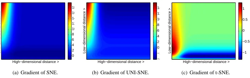
High−dimensional distance >

Low−dimensional distance >

0 2 4 6 8 10 12 14 16 18

(a) Gradient of SNE.

High−dimensional distance >

Low−dimensional distance >

−4 −2 0 2 4 6 8 10 12 14

(b) Gradient of UNI-SNE.

High−dimensional distance > Low−dimensional distance > −1

−0.5 0 0.5 1

(c) Gradient of t-SNE.

Figure 1: Gradients of three types of SNE as a function of the pairwise Euclidean distance between two points in the high-dimensional and the pairwise distance between the points in the low-dimensional data representation.

selection of the Student t-distribution is that it is closely related to the Gaussian distribution, as the Student t-distribution is an infinite mixture of Gaussians. A computationally convenient property is that it is much faster to evaluate the density of a point under a Student t-distribution than under a Gaussian because it does not involve an exponential, even though the Student t-distribution is equivalent to an infinite mixture of Gaussians with different variances.

The gradient of the Kullback-Leibler divergence between P and the Student-t based joint prob-ability distribution Q (computed using Equation 4) is derived in Appendix A, and is given by

δC

δyi

=4

∑

j

(pi j−qi j)(yi−yj) 1+kyi−yjk2

−1

. (5)

In Figure 1(a) to 1(c), we show the gradients between two low-dimensional datapoints yiand yjas

a function of their pairwise Euclidean distances in the high-dimensional and the low-dimensional space (i.e., as a function of_kxi−xjkandkyi−yjk) for the symmetric versions of SNE, UNI-SNE,

and t-SNE. In the figures, positive values of the gradient represent an attraction between the low-dimensional datapoints yi and yj, whereas negative values represent a repulsion between the two

datapoints. From the figures, we observe two main advantages of the t-SNE gradient over the gradients of SNE and UNI-SNE.

First, the t-SNE gradient strongly repels dissimilar datapoints that are modeled by a small pair-wise distance in the low-dimensional representation. SNE has such a repulsion as well, but its effect is minimal compared to the strong attractions elsewhere in the gradient (the largest attraction in our graphical representation of the gradient is approximately 19, whereas the largest repulsion is approx-imately 1). In UNI-SNE, the amount of repulsion between dissimilar datapoints is slightly larger, however, this repulsion is only strong when the pairwise distance between the points in the low-dimensional representation is already large (which is often not the case, since the low-low-dimensional representation is initialized by sampling from a Gaussian with a very small variance that is centered around the origin).

Algorithm 1: Simple version of t-Distributed Stochastic Neighbor Embedding. Data: data set

X

cost function parameters: perplexity Per p,

optimization parameters: number of iterations T , learning rateη, momentumα(t). Result: low-dimensional data representation

Y

begin

compute pairwise affinities pj|iwith perplexity Per p (using Equation 1)

set pi j= pj|i+pi|j

2n

sample initial solution

Y

N

for t=1 to T do

compute low-dimensional affinities qi j (using Equation 4)

compute gradient _δδC_Y (using Equation 5)

set

Y

Y

δY +α(t)

Y

Y

end end

is proportional to their pairwise distance in the low-dimensional map, which may cause dissimilar datapoints to move much too far away from each other.

Taken together, t-SNE puts emphasis on (1) modeling dissimilar datapoints by means of large pairwise distances, and (2) modeling similar datapoints by means of small pairwise distances. More-over, as a result of these characteristics of the t-SNE cost function (and as a result of the approximate scale invariance of the Student t-distribution), the optimization of the t-SNE cost function is much easier than the optimization of the cost functions of SNE and UNI-SNE. Specifically, t-SNE in-troduces long-range forces in the low-dimensional map that can pull back together two (clusters of) similar points that get separated early on in the optimization. SNE and UNI-SNE do not have such long-range forces, as a result of which SNE and UNI-SNE need to use simulated annealing to obtain reasonable solutions. Instead, the long-range forces in t-SNE facilitate the identification of good local optima without resorting to simulated annealing.

3.4 Optimization Methods for t-SNE

We start by presenting a relatively simple, gradient descent procedure for optimizing the t-SNE cost function. This simple procedure uses a momentum term to reduce the number of iterations required and it works best if the momentum term is small until the map points have become moderately well organized. Pseudocode for this simple algorithm is presented in Algorithm 1. The simple algorithm can be sped up using the adaptive learning rate scheme that is described by Jacobs (1988), which gradually increases the learning rate in directions in which the gradient is stable.

distances of the map points from the origin. The magnitude of this penalty term and the iteration at which it is removed are set by hand, but the behavior is fairly robust across variations in these two additional optimization parameters.

A less obvious way to improve the optimization, which we call “early exaggeration”, is to multiply all of the pi j’s by, for example, 4, in the initial stages of the optimization. This means that

almost all of the qi j’s, which still add up to 1, are much too small to model their corresponding pi j’s.

As a result, the optimization is encouraged to focus on modeling the large pi j’s by fairly large qi j’s.

The effect is that the natural clusters in the data tend to form tight widely separated clusters in the map. This creates a lot of relatively empty space in the map, which makes it much easier for the clusters to move around relative to one another in order to find a good global organization.

In all the visualizations presented in this paper and in the supporting material, we used exactly the same optimization procedure. We used the early exaggeration method with an exaggeration of 4 for the first 50 iterations (note that early exaggeration is not included in the pseudocode in Algorithm 1). The number of gradient descent iterations T was set 1000, and the momentum term was set toα(t)=0.5 for t<250 andα(t)=0.8 for t_≥250. The learning rateηis initially set to 100 and it is updated after every iteration by means of the adaptive learning rate scheme described by Jacobs (1988). A Matlab implementation of the resulting algorithm is available athttp://ticc. uvt.nl/˜lvdrmaaten/tsne.

4. Experiments

To evaluate t-SNE, we present experiments in which t-SNE is compared to seven other non-parametric techniques for dimensionality reduction. Because of space limitations, in the paper, we only com-pare t-SNE with: (1) Sammon mapping, (2) Isomap, and (3) LLE. In the supporting material, we also compare t-SNE with: (4) CCA, (5) SNE, (6) MVU, and (7) Laplacian Eigenmaps. We per-formed experiments on five data sets that represent a variety of application domains. Again because of space limitations, we restrict ourselves to three data sets in the paper. The results of our experi-ments on the remaining two data sets are presented in the supplemental material.

In Section 4.1, the data sets that we employed in our experiments are introduced. The setup of the experiments is presented in Section 4.2. In Section 4.3, we present the results of our experiments.

4.1 Data Sets

The five data sets we employed in our experiments are: (1) the MNIST data set, (2) the Olivetti faces data set, (3) the COIL-20 data set, (4) the word-features data set, and (5) the Netflix data set. We only present results on the first three data sets in this section. The results on the remaining two data sets are presented in the supporting material. The first three data sets are introduced below.

The MNIST data set6 contains 60,000 grayscale images of handwritten digits. For our experi-ments, we randomly selected 6,000 of the images for computational reasons. The digit images have 28_×28=784 pixels (i.e., dimensions). The Olivetti faces data set7consists of images of 40 indi-viduals with small variations in viewpoint, large variations in expression, and occasional addition of glasses. The data set consists of 400 images (10 per individual) of size 92_×112=10,304 pixels, and is labeled according to identity. The COIL-20 data set (Nene et al., 1996) contains images of 20

different objects viewed from 72 equally spaced orientations, yielding a total of 1,440 images. The images contain 32_×32=1,024 pixels.

4.2 Experimental Setup

In all of our experiments, we start by using PCA to reduce the dimensionality of the data to 30. This speeds up the computation of pairwise distances between the datapoints and suppresses some noise without severely distorting the interpoint distances. We then use each of the dimensionality reduction techniques to convert the 30-dimensional representation to a two-dimensional map and we show the resulting map as a scatterplot. For all of the data sets, there is information about the class of each datapoint, but the class information is only used to select a color and/or symbol for the map points. The class information is not used to determine the spatial coordinates of the map points. The coloring thus provides a way of evaluating how well the map preserves the similarities within each class.

The cost function parameter settings we employed in our experiments are listed in Table 1. In the table, Per p represents the perplexity of the conditional probability distribution induced by a Gaussian kernel and k represents the number of nearest neighbors employed in a neighborhood graph. In the experiments with Isomap and LLE, we only visualize datapoints that correspond to vertices in the largest connected component of the neighborhood graph.8For the Sammon mapping optimization, we performed Newton’s method for 500 iterations.

Technique Cost function parameters

t-SNE Per p=40

Sammon mapping none

Isomap k=12

LLE k=12

Table 1: Cost function parameter settings for the experiments.

4.3 Results

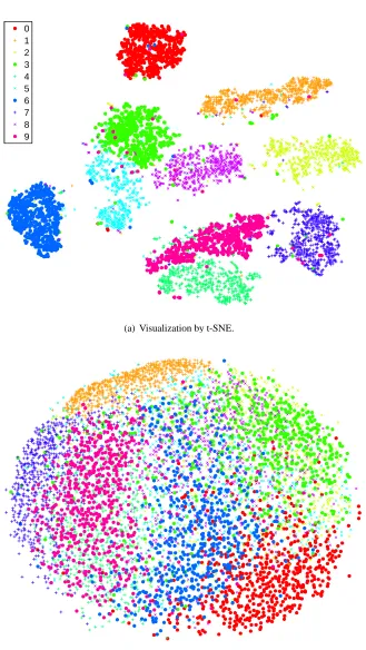
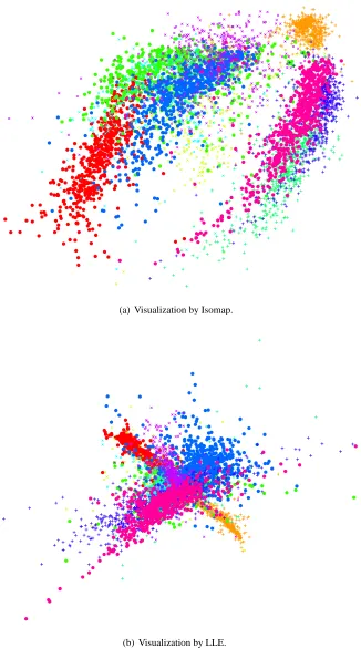
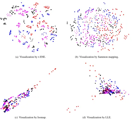
In Figures 2 and 3, we show the results of our experiments with t-SNE, Sammon mapping, Isomap, and LLE on the MNIST data set. The results reveal the strong performance of t-SNE compared to the other techniques. In particular, Sammon mapping constructs a “ball” in which only three classes (representing the digits 0, 1, and 7) are somewhat separated from the other classes. Isomap and LLE produce solutions in which there are large overlaps between the digit classes. In contrast, t-SNE constructs a map in which the separation between the digit classes is almost perfect. Moreover, detailed inspection of the t-SNE map reveals that much of the local structure of the data (such as the orientation of the ones) is captured as well. This is illustrated in more detail in Section 5 (see Figure 7). The map produced by t-SNE contains some points that are clustered with the wrong class, but most of these points correspond to distorted digits many of which are difficult to identify. Figure 4 shows the results of applying t-SNE, Sammon mapping, Isomap, and LLE to the Olivetti faces data set. Again, Isomap and LLE produce solutions that provide little insight into the class

0 1 2 3 4 5 6 7 8 9

(a) Visualization by t-SNE.

(b) Visualization by Sammon mapping.

(a) Visualization by Isomap.

(b) Visualization by LLE.

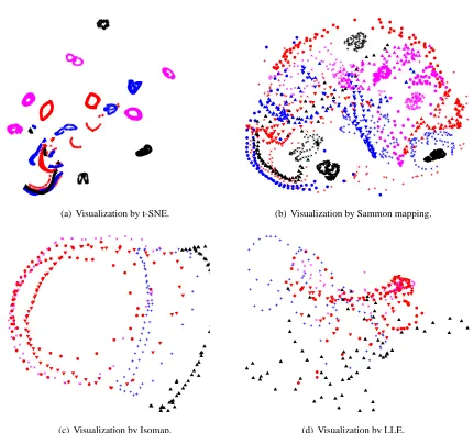
(a) Visualization by t-SNE. (b) Visualization by Sammon mapping.

(c) Visualization by Isomap. (d) Visualization by LLE.

Figure 4: Visualizations of the Olivetti faces data set.

structure of the data. The map constructed by Sammon mapping is significantly better, since it models many of the members of each class fairly close together, but none of the classes are clearly separated in the Sammon map. In contrast, t-SNE does a much better job of revealing the natural classes in the data. Some individuals have their ten images split into two clusters, usually because a subset of the images have the head facing in a significantly different direction, or because they have a very different expression or glasses. For these individuals, it is not clear that their ten images form a natural class when using Euclidean distance in pixel space.

(a) Visualization by t-SNE. (b) Visualization by Sammon mapping.

(c) Visualization by Isomap. (d) Visualization by LLE.

Figure 5: Visualizations of the COIL-20 data set.

similarity between different cars at the same orientation. This prevents t-SNE from keeping the four manifolds clearly separate. Figure 5 also reveals that the other three techniques are not nearly as good at cleanly separating the manifolds that correspond to very different objects. In addition, Isomap and LLE only visualize a small number of classes from the COIL-20 data set, because the data set comprises a large number of widely separated submanifolds that give rise to small connected components in the neighborhood graph.

5. Applying t-SNE to Large Data Sets

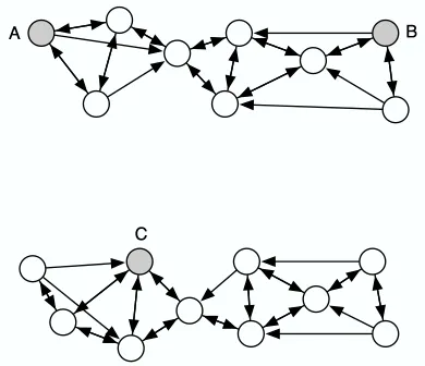
Figure 6: An illustration of the advantage of the random walk version of t-SNE over a standard landmark approach. The shaded points A, B, and C are three (almost) equidistant land-mark points, whereas the non-shaded datapoints are non-landland-mark points. The arrows represent a directed neighborhood graph where k=3. In a standard landmark approach, the pairwise affinity between A and B is approximately equal to the pairwise affinity be-tween A and C. In the random walk version of t-SNE, the pairwise affinity bebe-tween A and B is much larger than the pairwise affinity between A and C, and therefore, it reflects the structure of the data much better.

make use of the information that the undisplayed datapoints provide about the underlying manifolds. Suppose, for example, that A, B, and C are all equidistant in the high-dimensional space. If there are many undisplayed datapoints between A and B and none between A and C, it is much more likely that A and B are part of the same cluster than A and C. This is illustrated in Figure 6. In this section, we show how t-SNE can be modified to display a random subset of the datapoints (so-called landmark points) in a way that uses information from the entire (possibly very large) data set.

We start by choosing a desired number of neighbors and creating a neighborhood graph for all of the datapoints. Although this is computationally intensive, it is only done once. Then, for each of the landmark points, we define a random walk starting at that landmark point and terminating as soon as it lands on another landmark point. During a random walk, the probability of choosing an edge emanating from node xi to node xj is proportional to e−kxi−xjk

2

. We define pj_|i to be the

fraction of random walks starting at landmark point xi that terminate at landmark point xj. This has

The most obvious way to compute the random walk-based similarities pj|iis to explicitly

per-form the random walks on the neighborhood graph, which works very well in practice, given that one can easily perform one million random walks per second. Alternatively, Grady (2006) presents an analytical solution to compute the pairwise similarities pj|i that involves solving a sparse linear

system. The analytical solution to compute the similarities pj|iis sketched in Appendix B. In

pre-liminary experiments, we did not find significant differences between performing the random walks explicitly and the analytical solution. In the experiment we present below, we explicitly performed the random walks because this is computationally less expensive. However, for very large data sets in which the landmark points are very sparse, the analytical solution may be more appropriate.

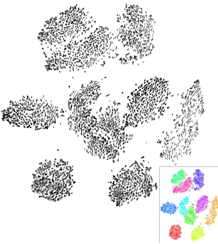
Figure 7 shows the results of an experiment, in which we applied the random walk version of t-SNE to 6,000 randomly selected digits from the MNIST data set, using all 60,000 digits to compute the pairwise affinities pj_|i. In the experiment, we used a neighborhood graph that was

constructed using a value of k=20 nearest neighbors.9 _{The inset of the figure shows the same} visualization as a scatterplot in which the colors represent the labels of the digits. In the t-SNE map, all classes are clearly separated and the “continental” sevens form a small separate cluster. Moreover, t-SNE reveals the main dimensions of variation within each class, such as the orientation of the ones, fours, sevens, and nines, or the “loopiness” of the twos. The strong performance of t-SNE is also reflected in the generalization error of nearest neighbor classifiers that are trained on the low-dimensional representation. Whereas the generalization error (measured using 10-fold cross validation) of a 1-nearest neighbor classifier trained on the original 784-dimensional datapoints is 5.75%, the generalization error of a 1-nearest neighbor classifier trained on the two-dimensional data representation produced by t-SNE is only 5.13%. The computational requirements of random walk t-SNE are reasonable: it took only one hour of CPU time to construct the map in Figure 7.

6. Discussion

The results in the previous two sections (and those in the supplemental material) demonstrate the performance of t-SNE on a wide variety of data sets. In this section, we discuss the differences between t-SNE and other non-parametric techniques (Section 6.1), and we also discuss a number of weaknesses and possible improvements of t-SNE (Section 6.2).

6.1 Comparison with Related Techniques

Classical scaling (Torgerson, 1952), which is closely related to PCA (Mardia et al., 1979; Williams, 2002), finds a linear transformation of the data that minimizes the sum of the squared errors between high-dimensional pairwise distances and their low-dimensional representatives. A linear method such as classical scaling is not good at modeling curved manifolds and it focuses on preserving the distances between widely separated datapoints rather than on preserving the distances between nearby datapoints. An important approach that attempts to address the problems of classical scaling is the Sammon mapping (Sammon, 1969) which alters the cost function of classical scaling by dividing the squared error in the representation of each pairwise Euclidean distance by the original Euclidean distance in the high-dimensional space. The resulting cost function is given by

C= 1

∑i jkxi−xjk_i

∑

(_kxi−xjk − kyi−yjk)2 kxi−xjk

,

where the constant outside of the sum is added in order to simplify the derivation of the gradient. The main weakness of the Sammon cost function is that the importance of retaining small pairwise distances in the map is largely dependent on small differences in these pairwise distances. In par-ticular, a small error in the model of two high-dimensional points that are extremely close together results in a large contribution to the cost function. Since all small pairwise distances constitute the local structure of the data, it seems more appropriate to aim to assign approximately equal impor-tance to all small pairwise disimpor-tances.

In contrast to Sammon mapping, the Gaussian kernel employed in the high-dimensional space by t-SNE defines a soft border between the local and global structure of the data and for pairs of datapoints that are close together relative to the standard deviation of the Gaussian, the impor-tance of modeling their separations is almost independent of the magnitudes of those separations. Moreover, t-SNE determines the local neighborhood size for each datapoint separately based on the local density of the data (by forcing each conditional probability distribution Pi to have the same

perplexity).

The strong performance of t-SNE compared to Isomap is partly explained by Isomap’s suscep-tibility to “short-circuiting”. Also, Isomap mainly focuses on modeling large geodesic distances rather than small ones.

The strong performance of t-SNE compared to LLE is mainly due to a basic weakness of LLE: the only thing that prevents all datapoints from collapsing onto a single point is a constraint on the covariance of the low-dimensional representation. In practice, this constraint is often satisfied by placing most of the map points near the center of the map and using a few widely scattered points to create large covariance (see Figure 3(b) and 4(d)). For neighborhood graphs that are almost disconnected, the covariance constraint can also be satisfied by a “curdled” map in which there are a few widely separated, collapsed subsets corresponding to the almost disconnected components. Furthermore, neighborhood-graph based techniques (such as Isomap and LLE) are not capable of visualizing data that consists of two or more widely separated submanifolds, because such data does not give rise to a connected neighborhood graph. It is possible to produce a separate map for each connected component, but this loses information about the relative similarities of the separate components.

Like Isomap and LLE, the random walk version of t-SNE employs neighborhood graphs, but it does not suffer from short-circuiting problems because the pairwise similarities between the high-dimensional datapoints are computed by integrating over all paths through the neighborhood graph. Because of the diffusion-based interpretation of the conditional probabilities underlying the random walk version of t-SNE, it is useful to compare t-SNE to diffusion maps. Diffusion maps define a “diffusion distance” on the high-dimensional datapoints that is given by

D(t)(xi,xj) =

v u u u t

∑

k

p(_ikt)−p(_jkt) 2

ψ(xk)(0) ,

where p(_{i j}t) represents the probability of a particle traveling from xi to xj in t timesteps through a

graph on the data with Gaussian emission probabilities. The termψ(xk)(0)is a measure for the local

eigenvec-tors are employed, the Euclidean distances in the diffusion map are equal to the diffusion distances in the high-dimensional data representation (Lafon and Lee, 2006). Mathematically, diffusion maps minimize

C=

∑

i

∑

D(t)(xi,xj)− kyi−yjk

2

.

As a result, diffusion maps are susceptible to the same problems as classical scaling: they assign much higher importance to modeling the large pairwise diffusion distances than the small ones and as a result, they are not good at retaining the local structure of the data. Moreover, in contrast to the random walk version of t-SNE, diffusion maps do not have a natural way of selecting the length, t, of the random walks.

In the supplemental material, we present results that reveal that t-SNE outperforms CCA (De-martines and H´erault, 1997), MVU (Weinberger et al., 2004), and Laplacian Eigenmaps (Belkin and Niyogi, 2002) as well. For CCA and the closely related CDA (Lee et al., 2000), these results can be partially explained by the hard borderλthat these techniques define between local and global structure, as opposed to the soft border of t-SNE. Moreover, within the rangeλ, CCA suffers from the same weakness as Sammon mapping: it assigns extremely high importance to modeling the distance between two datapoints that are extremely close.

Like t-SNE, MVU (Weinberger et al., 2004) tries to model all of the small separations well but MVU insists on modeling them perfectly (i.e., it treats them as constraints) and a single erroneous constraint may severely affect the performance of MVU. This can occur when there is a short-circuit between two parts of a curved manifold that are far apart in the intrinsic manifold coordinates. Also, MVU makes no attempt to model longer range structure: It simply pulls the map points as far apart as possible subject to the hard constraints so, unlike t-SNE, it cannot be expected to produce sensible large-scale structure in the map.

For Laplacian Eigenmaps, the poor results relative to t-SNE may be explained by the fact that Laplacian Eigenmaps have the same covariance constraint as LLE, and it is easy to cheat on this constraint.

6.2 Weaknesses

Although we have shown that SNE compares favorably to other techniques for data visualization, t-SNE has three potential weaknesses: (1) it is unclear how t-t-SNE performs on general dimensionality reduction tasks, (2) the relatively local nature of t-SNE makes it sensitive to the curse of the intrinsic dimensionality of the data, and (3) t-SNE is not guaranteed to converge to a global optimum of its cost function. Below, we discuss the three weaknesses in more detail.

in which the dimensionality of the data needs to be reduced to a dimensionality higher than three, Student t-distributions with more than one degree of freedom10are likely to be more appropriate.

2) Curse of intrinsic dimensionality. t-SNE reduces the dimensionality of data mainly based on local properties of the data, which makes t-SNE sensitive to the curse of the intrinsic dimensional-ity of the data (Bengio, 2007). In data sets with a high intrinsic dimensionaldimensional-ity and an underlying manifold that is highly varying, the local linearity assumption on the manifold that t-SNE implicitly makes (by employing Euclidean distances between near neighbors) may be violated. As a result, t-SNE might be less successful if it is applied on data sets with a very high intrinsic dimensional-ity (for instance, a recent study by Meytlis and Sirovich (2007) estimates the space of images of faces to be constituted of approximately 100 dimensions). Manifold learners such as Isomap and LLE suffer from exactly the same problems (see, e.g., Bengio, 2007; van der Maaten et al., 2008). A possible way to (partially) address this issue is by performing t-SNE on a data representation obtained from a model that represents the highly varying data manifold efficiently in a number of nonlinear layers such as an autoencoder (Hinton and Salakhutdinov, 2006). Such deep-layer archi-tectures can represent complex nonlinear functions in a much simpler way, and as a result, require fewer datapoints to learn an appropriate solution (as is illustrated for a d-bits parity task by Bengio 2007). Performing t-SNE on a data representation produced by, for example, an autoencoder is likely to improve the quality of the constructed visualizations, because autoencoders can identify highly-varying manifolds better than a local method such as t-SNE. However, the reader should note that it is by definition impossible to fully represent the structure of intrinsically high-dimensional data in two or three dimensions.

3) Non-convexity of the t-SNE cost function. A nice property of most state-of-the-art dimen-sionality reduction techniques (such as classical scaling, Isomap, LLE, and diffusion maps) is the convexity of their cost functions. A major weakness of t-SNE is that the cost function is not convex, as a result of which several optimization parameters need to be chosen. The constructed solutions depend on these choices of optimization parameters and may be different each time t-SNE is run from an initial random configuration of map points. We have demonstrated that the same choice of optimization parameters can be used for a variety of different visualization tasks, and we found that the quality of the optima does not vary much from run to run. Therefore, we think that the weakness of the optimization method is insufficient reason to reject t-SNE in favor of methods that lead to con-vex optimization problems but produce noticeably worse visualizations. A local optimum of a cost function that accurately captures what we want in a visualization is often preferable to the global optimum of a cost function that fails to capture important aspects of what we want. Moreover, the convexity of cost functions can be misleading, because their optimization is often computationally infeasible for large real-world data sets, prompting the use of approximation techniques (de Silva and Tenenbaum, 2003; Weinberger et al., 2007). Even for LLE and Laplacian Eigenmaps, the opti-mization is performed using iterative Arnoldi (Arnoldi, 1951) or Jacobi-Davidson (Fokkema et al., 1999) methods, which may fail to find the global optimum due to convergence problems.

7. Conclusions

The paper presents a new technique for the visualization of similarity data that is capable of retaining the local structure of the data while also revealing some important global structure (such as clusters

at multiple scales). Both the computational and the memory complexity of t-SNE are O(n2_{), but} we present a landmark approach that makes it possible to successfully visualize large real-world data sets with limited computational demands. Our experiments on a variety of data sets show that t-SNE outperforms existing state-of-the-art techniques for visualizing a variety of real-world data sets. Matlab implementations of both the normal and the random walk version of t-SNE are available for download athttp://ticc.uvt.nl/˜lvdrmaaten/tsne.

In future work we plan to investigate the optimization of the number of degrees of freedom of the Student-t distribution used in t-SNE. This may be helpful for dimensionality reduction when the low-dimensional representation has many dimensions. We will also investigate the extension of t-SNE to models in which each high-dimensional datapoint is modeled by several low-dimensional map points as in Cook et al. (2007). Also, we aim to develop a parametric version of t-SNE that allows for generalization to held-out test data by using the t-SNE objective function to train a mul-tilayer neural network that provides an explicit mapping to the low-dimensional space.

Acknowledgments

The authors thank Sam Roweis for many helpful discussions, Andriy Mnih for supplying the word-features data set, Ruslan Salakhutdinov for help with the Netflix data set (results for these data sets are presented in the supplemental material), and Guido de Croon for pointing us to the analytical solution of the random walk probabilities.

Laurens van der Maaten is supported by the CATCH-programme of the Dutch Scientific Orga-nization (NWO), project RICH (grant 640.002.401), and cooperates with RACM. Geoffrey Hinton is a fellow of the Canadian Institute for Advanced Research, and is also supported by grants from NSERC and CFI and gifts from Google and Microsoft.

Appendix A. Derivation of the t-SNE gradient

t-SNE minimizes the Kullback-Leibler divergence between the joint probabilities pi j in the

high-dimensional space and the joint probabilities qi jin the low-dimensional space. The values of pi jare

defined to be the symmetrized conditional probabilities, whereas the values of qi j are obtained by

means of a Student-t distribution with one degree of freedom

pi j=

pj|i+pi|j

2n ,

qi j=

1+_kyi−yjk2

−1

∑k6=l(1+kyk−ylk2)−1 ,

where p_j|iand p_i|jare either obtained from Equation 1 or from the random walk procedure described in Section 5. The values of piiand qiiare set to zero. The Kullback-Leibler divergence between the

two joint probability distributions P and Q is given by

C=KL(P_||Q) =

∑

i

∑

pi jlog

pi j

qi j

=

∑

i

∑

In order to make the derivation less cluttered, we define two auxiliary variables di jand Z as follows

di j=kyi−yjk,

Z=

∑

k6=l

(1+d_kl2)−1_.

Note that if yi changes, the only pairwise distances that change are di j and djifor∀j. Hence, the

gradient of the cost function C with respect to yiis given by

δC

δyi

=

∑

j

δ C

δdi j

+_δδC dji

(yi−yj)

=2

∑

j δC

δdi j

(yi−yj). (7)

The gradient _δδ_dC

i j is computed from the definition of the Kullback-Leibler divergence in Equation 6

(note that the first part of this equation is a constant).

δC

δdi j

=₋

∑

k6=l

pkl

δ(log qkl) δdi j

=₋

∑

k6=l

pkl

δ(log qklZ−log Z) δdi j

=₋

∑

k6=l

pkl

1 qklZ

δ((1+d2_kl)−1₎

δdi j −

1 Z

δZ

δdi j

The gradient δ((1+dkl2)−1)

δdi j is only nonzero when k=i and l= j. Hence, the gradient

δC

δdi j is given by

δC

δdi j

=2 pi j qi jZ

(1+d_{i j}2)−2₋2

∑

k6=l

pkl

(1+d2

i j)−2

Z .

Noting that∑k6=lpkl=1, we see that the gradient simplifies to

δC

δdi j

=2pi j(1+di j2)−1−2qi j(1+di j2)−1

=2(pi j−qi j)(1+di j2)−1.

Substituting this term into Equation 7, we obtain the gradient

δC

δyi

=4

∑

j

(pi j−qi j)(1+kyi−yjk2)−1(yi−yj).

Appendix B. Analytical Solution to Random Walk Probabilities

It can be shown that computing the probability that a random walk initiated from a non-landmark point (on a graph that is specified by adjacency matrix W ) first reaches a specific landmark point is equal to computing the solution to the combinatorial Dirichlet problem in which the boundary conditions are at the locations of the landmark points, the considered landmark point is fixed to unity, and the other landmarks points are set to zero (Kakutani, 1945; Doyle and Snell, 1984). In practice, the solution can thus be obtained by minimizing the combinatorial formulation of the Dirichlet integral

D[x] =1 2x

T_Lx,

where L represents the graph Laplacian. Mathematically, the graph Laplacian is given by L= D−W , where D=diag ∑jw1 j,∑jw2 j, ...,∑jwn j

. Without loss of generality, we may reorder the landmark points such that the landmark points come first. As a result, the combinatorial Dirichlet integral decomposes into

D[xN] =

1 2

xT_L xT_N

LL B

BT LN

xL

xN

=1 2 x

T

LLLxL+2xNTBTxM+xTNLNxN

,

where we use the subscript_·L to indicate the landmark points, and the subscript·N to indicate the

non-landmark points. Differentiating D[xN]with respect to xNand finding its critical points amounts

to solving the linear systems

LNxN=−BT. (8)

Please note that in this linear system, BT is a matrix containing the columns from the graph Lapla-cian L that correspond to the landmark points (excluding the rows that correspond to landmark points). After normalization of the solutions to the systems XN, the column vectors of XN contain

the probability that a random walk initiated from a non-landmark point terminates in a landmark point. One should note that the linear system in Equation 8 is only nonsingular if the graph is com-pletely connected, or if each connected component in the graph contains at least one landmark point (Biggs, 1974).

Because we are interested in the probability of a random walk initiated from a landmark point terminating at another landmark point, we duplicate all landmark points in the neighborhood graph, and initiate the random walks from the duplicate landmarks. Because of memory constraints, it is not possible to store the entire matrix XN into memory (note that we are only interested in a small

number of rows from this matrix, viz., in the rows corresponding to the duplicate landmark points). Hence, we solve the linear systems defined by the columns of₋BT one-by-one, and store only the parts of the solutions that correspond to the duplicate landmark points. For computational reasons, we first perform a Cholesky factorization of LN, such that LN=CCT, where C is an upper-triangular

matrix. Subsequently, the solution to the linear system in Equation 8 is obtained by solving the linear systems Cy=₋BT and CxN=y using a fast backsubstitution method.

References

G.D. Battista, P. Eades, R. Tamassia, and I.G. Tollis. Annotated bibliography on graph drawing. Computational Geometry: Theory and Applications, 4:235–282, 1994.

M. Belkin and P. Niyogi. Laplacian Eigenmaps and spectral techniques for embedding and cluster-ing. In Advances in Neural Information Processing Systems, volume 14, pages 585–591, Cam-bridge, MA, USA, 2002. The MIT Press.

Y. Bengio. Learning deep architectures for AI. Technical Report 1312, Universit ´e de Montr´eal, 2007.

N. Biggs. Algebraic graph theory. In Cambridge Tracts in Mathematics, volume 67. Cambridge University Press, 1974.

H. Chernoff. The use of faces to represent points in k-dimensional space graphically. Journal of the American Statistical Association, 68:361–368, 1973.

J.A. Cook, I. Sutskever, A. Mnih, and G.E. Hinton. Visualizing similarity data with a mixture of maps. In Proceedings of the 11thInternational Conference on Artificial Intelligence and Statistics, volume 2, pages 67–74, 2007.

M.C. Ferreira de Oliveira and H. Levkowitz. From visual data exploration to visual data mining: A survey. IEEE Transactions on Visualization and Computer Graphics, 9(3):378–394, 2003.

V. de Silva and J.B. Tenenbaum. Global versus local methods in nonlinear dimensionality reduction. In Advances in Neural Information Processing Systems, volume 15, pages 721–728, Cambridge, MA, USA, 2003. The MIT Press.

P. Demartines and J. H´erault. Curvilinear component analysis: A self-organizing neural network for nonlinear mapping of data sets. IEEE Transactions on Neural Networks, 8(1):148–154, 1997.

P. Doyle and L. Snell. Random walks and electric networks. In Carus mathematical monographs, volume 22. Mathematical Association of America, 1984.

D.R. Fokkema, G.L.G. Sleijpen, and H.A. van der Vorst. Jacobi–Davidson style QR and QZ algo-rithms for the reduction of matrix pencils. SIAM Journal on Scientific Computing, 20(1):94–125, 1999.

L. Grady. Random walks for image segmentation. IEEE Transactions on Pattern Analysis and Machine Intelligence, 28(11):1768–1783, 2006.

G.E. Hinton and S.T. Roweis. Stochastic Neighbor Embedding. In Advances in Neural Information Processing Systems, volume 15, pages 833–840, Cambridge, MA, USA, 2002. The MIT Press.

G.E. Hinton and R.R. Salakhutdinov. Reducing the dimensionality of data with neural networks. Science, 313(5786):504–507, 2006.

H. Hotelling. Analysis of a complex of statistical variables into principal components. Journal of Educational Psychology, 24:417–441, 1933.

S. Kakutani. Markov processes and the Dirichlet problem. Proceedings of the Japan Academy, 21: 227–233, 1945.

D.A. Keim. Designing pixel-oriented visualization techniques: Theory and applications. IEEE Transactions on Visualization and Computer Graphics, 6(1):59–78, 2000.

S. Lafon and A.B. Lee. Diffusion maps and coarse-graining: A unified framework for dimension-ality reduction, graph partitioning, and data set parameterization. IEEE Transactions on Pattern Analysis and Machine Intelligence, 28(9):1393–1403, 2006.

J.A. Lee and M. Verleysen. Nonlinear dimensionality reduction of data manifolds with essential loops. Neurocomputing, 67:29–53, 2005.

J.A. Lee and M. Verleysen. Nonlinear dimensionality reduction. Springer, New York, NY, USA, 2007.

J.A. Lee, A. Lendasse, N. Donckers, and M. Verleysen. A robust nonlinear projection method. In Proceedings of the 8thEuropean Symposium on Artificial Neural Networks, pages 13–20, 2000.

K.V. Mardia, J.T. Kent, and J.M. Bibby. Multivariate Analysis. Academic Press, 1979.

M. Meytlis and L. Sirovich. On the dimensionality of face space. IEEE Transactions of Pattern Analysis and Machine Intelligence, 29(7):1262–1267, 2007.

B. Nadler, S. Lafon, R.R. Coifman, and I.G. Kevrekidis. Diffusion maps, spectral clustering and the reaction coordinates of dynamical systems. Applied and Computational Harmonic Analysis: Special Issue on Diffusion Maps and Wavelets, 21:113–127, 2006.

S.A. Nene, S.K. Nayar, and H. Murase. Columbia Object Image Library (COIL-20). Technical Report CUCS-005-96, Columbia University, 1996.

S.T. Roweis and L.K. Saul. Nonlinear dimensionality reduction by Locally Linear Embedding. Science, 290(5500):2323–2326, 2000.

J.W. Sammon. A nonlinear mapping for data structure analysis. IEEE Transactions on Computers, 18(5):401–409, 1969.

L. Song, A.J. Smola, K. Borgwardt, and A. Gretton. Colored Maximum Variance Unfolding. In Advances in Neural Information Processing Systems, volume 21 (in press), 2007.

W.N. Street, W.H. Wolberg, and O.L. Mangasarian. Nuclear feature extraction for breast tumor diagnosis. In Proceedings of the IS&T/SPIE International Symposium on Electronic Imaging: Science and Technology, volume 1905, pages 861–870, 1993.

M. Szummer and T. Jaakkola. Partially labeled classification with Markov random walks. In Ad-vances in Neural Information Processing Systems, volume 14, pages 945–952, 2001.

W.S. Torgerson. Multidimensional scaling I: Theory and method. Psychometrika, 17:401–419, 1952.

L.J.P. van der Maaten, E.O. Postma, and H.J. van den Herik. Dimensionality reduction: A compar-ative review. Online Preprint, 2008.

K.Q. Weinberger, F. Sha, and L.K. Saul. Learning a kernel matrix for nonlinear dimensionality reduction. In Proceedings of the 21st International Confernence on Machine Learning, 2004.

K.Q. Weinberger, F. Sha, Q. Zhu, and L.K. Saul. Graph Laplacian regularization for large-scale semidefinite programming. In Advances in Neural Information Processing Systems, volume 19, 2007.

C.K.I. Williams. On a connection between Kernel PCA and metric multidimensional scaling. Ma-chine Learning, 46(1-3):11–19, 2002.