Study on Computer Generated Electromagnetic Effects on Computer Users

867

Copyright © 2011-15. Vandana Publications. All Rights Reserved.

Volume-5, Issue-2, April-2015

International Journal of Engineering and Management Research

Page Number: 867-872

Optimization of Process Parameters of GMAW using TLBO Technique

Gaurav S. Sharma1,S.L. Shinde2, R.S. Sayare3 1,2,3

Department of Mechanical Engineering, INDIA

ABSTRACT

In this paper, the optimization of bead geometry using TLBO technique is presented which includes the effect of welding parameters like wire feed rate, welding voltage, welding speed and gas flow rate on bead geometry parameters of AISI 430 grade stainless steel material during welding. A plan of A plan of experiments based on TLBO technique has been used to acquire the data. Central composite Design Matrix and analysis of variance (ANOVA) are employed to investigate the bead geometry parameters of AISI 430 grade SS material & optimize the bead geometry parameters. Finally the conformations tests have been carried out to compare the predicated values with the experimental values confirm its effectiveness in the analysis of penetration.

Keywords--- GMAW, Central composite design matrix, TLBO, etc

I.

INTRODUCTION

Quality is a vital factor in today’s manufacturing world. Quality can be defined as the degree of customer satisfaction. Quality of a product depends on how it performs in desired circumstances. Quality is a very vital factor in the field of welding. The quality of a weld depends on mechanical properties of the weld metal which in turn depends on metallurgical characteristics and chemical composition of the weld. The mechanical and metallurgical feature of weld depends on bead geometry which is directly related to welding process parameters. In other words quality of weld depends on input process parameters. GMA welding is a multi-objective and multifactor metal fabrication technique. The process parameters have a direct influence on bead geometry. Mechanical strength of weld metal is highly influenced by the composition of metal but also by weld bead shape. This is an indication of bead geometry. It mainly depends on wire feed rate, welding speed, arc voltage etc. Therefore it is necessary to study the relationship between input process parameters and bead parameters to study weld

bead geometry. This paper highlights the study carried out to develop mathematical models to predict weld bead geometry, in stainless steel cladding deposited by GMAW. In this project study Teaching Learning Based Optimization (TLBO) method is used to optimize the input process parameter of semi-automatic gas metal arc welding like welding speed (S), voltage (V), wire feed rate (F), gas flow rate (G) and getting optimum solution of welding geometry such as bead height (BH), bead width (BW), bead penetration (BP).

II.

EXPERIMENTAL PROCEDURE

The following machines and consumables were used for the purpose of conducting experiment.

1) Gas metal arc welding machine. 2) Welding manipulator.

3) Wire feeder.

4) Filler material Stainless Steel wire of 1.2 mm diameter (ER – 309L).

5) Gas cylinder containing a mixture of 98% argon and 2% of oxygen.

6) Stainless steel plate (AISI 430 grade).

868

Copyright © 2011-15. Vandana Publications. All Rights Reserved.

In this work, the four process parameters of GMAW process each at five levels have been decided for welding AISI 430 grade steel. These are very important controllable process parameters which will effects on weld bead and good appearance of weld bead. It is desirable to have five minimum levels of process parameters to reflect the true behavior of response parameters. The working ranges of the parameter are chosen by rough trials for a smooth appearance of weld bead. If the working ranges are smaller or larger the limits, then proper weld bead will not appear. The upper and lower limits of parameters are coded as +2 and -2 respectively. The coded values for intermediate ranges are calculated using the following equation (1):

i

X

x

+

x

(

x

−

x

(1)

where Xi is the required coded value of a variable X and is any value of the variable from Xmin to Xmax. The selected process parameters with their limits and notations are given in Table 2.

The central composite design matrix for conducting the experiments consist of 28 sets of trials. This design matrix depend on number of input process (k) and comprises of four Centre points (equal to number of input process parameters) and eight star points (twice the number of input process parameters) and sixteen factorial designs (2K

Expt. No.

), where 2 is the number of levels. The first 16 rows correspond to factorial portion, the row from 17 to 24 correspond to star point’s position and last 4 rows from 25 to 28 correspond to centre point’s position. Hence, final experimental design consist of 28 (i.e. 16+08+04= 28) trial and given in table 3.

Table: 3 Central composite design matrix

Wire feed rate

(F)

Welding Speed

(S)

Welding Voltage (V)

Gas flow rate (G)

1 -1 -1 -1 -1

2 -1 -1 -1 1

3 -1 -1 1 -1

4 -1 -1 1 1

5 -1 1 -1 -1

6 -1 1 -1 1

7 -1 1 1 -1

8 -1 1 1 1

9 1 -1 -1 -1

10 1 -1 -1 1

11 1 -1 1 -1

12 1 -1 1 1

13 1 1 -1 -1

14 1 1 -1 1

15 1 1 1 -1

16 1 1 1 1

17 -2 0 0 0

18 2 0 0 0

19 0 -2 0 0

20 0 2 0 0

21 0 0 -2 0

22 0 0 2 0

23 0 0 0 -2

24 0 0 0 2

25 0 0 0 0

26 0 0 0 0

27 0 0 0 0

28 0 0 0 0

III. MATHEMATICAL MODEL

869

Copyright © 2011-15. Vandana Publications. All Rights Reserved.

the relationships between the output parameters Y (BH, BW and BP) and input parameters (V, F, S and G). The second order response surface model for the four selected parameters is given by the equation (2).

Y=b0

∑

=

4

1

i

+ bixi

∑

=

4

1

i

+ biixi2

∑

≠=

4

1 ,

i j

j i

+ bijxixj (2)

For four parameters, the selected polynomial

could be expressed as given below (3): Y= b0+b1S+b2V+b3F+b4G +b11S2+b22V2+b33F2+b44G2 +

b12SV+b13SF+b14SG +b23VF+b24VG+b34FG (3)

Where, b0 is the free term of regression equation, b1,b2,...,bk are the linear terms, b11,b22,...,bkk are the quadratic terms and b12,b13,...,bk-1k are the interaction term. To test the goodness of the fit of the developed models, adequacy is determined by the Analysis of Variance technique (ANOVA). It is performed to evaluate the statistical significance of the fitted models and variables involved therein for response variable like BW, BH and BP. The values of “Probability >F” for model is less than 0.05 indicates that model is significant. The ANOVA for BH, BW and BP models are shown in Table 5, 6 and 7 respectively. It shows that the four main effects of the F, S, V, G parameters, six interactions of the FS, SV, SG, FV, VG, FG and four second-order effect of F2, S2, G2 and V2 are the most significant model terms. The values of significant coefficients for these models terms are calculated with the help of SYSTAT12 statistical software. The criterion used to illustrate the adequacy of a fitted model is multiple R2 and adjusted R2. The coefficient of determination R2 indicates the goodness of fit for the models, which provides a measure of variability in the observed response values and can be explained by the controllable parameters and their interactions. In BH, BW and BP, all the values of coefficient of determination R2 are nearly equal to 1. Clearly, we must have 0≤R2≤1, with larger values being more desirable. The adjusted R2 is a variation of the ordinary R2

BW=

299.61216.169F+0.034S6.836V18.042G+2.531F2+0.001S2+0.068V2+0.474G20.027FS

-0.005SV+0.007SG+0.332FV+0.094VG-0.492FG

(5)

statistic that reflects the number of parameters in the model. The entire adequacy measures are closer to 1, which is in reasonable agreement and indicate adequate models. The final mathematical models in uncoded form are given below:

BH=

213.573-25.557F-0.584S-4.264V-

0.094G+4.185F2+0.003S2+0.068V2+0.135G2+0.034FS-0.008SV+0.027SG-0.319FV+0.062VG+0.603FG (4)

BP = -133.593+47.474F-0.343S+1.128V+7.282G-3.290

F2+0.003S2-0.022V2-0.117G2+0.034FS+0.007SV-0.017SG-0.268FV+0.038VG-1.212FG

(6)

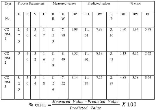
To verify the mathematical models, three experiments are conducted using different values of input process parameters in their working ranges but other than the values used in the design matrix. The output responses measured and the predicted results obtained are presented in Table 7. It is observed that the percentage error obtained between the measured and predicted values are quite small and the verification is satisfactory.

The weld bead volume (WBV) is a function of BH, BW and BP. Therefore, combine objective function is given as (7)

(WBV)min = 𝑤𝑤₁ 𝐵𝐵𝐵𝐵 𝐵𝐵𝐵𝐵𝑚𝑚𝑚𝑚𝑚𝑚 + 𝑤𝑤2

𝐵𝐵𝐵𝐵 𝐵𝐵𝐵𝐵𝑚𝑚𝑚𝑚𝑚𝑚 - 𝑤𝑤3

𝐵𝐵𝐵𝐵 𝐵𝐵𝐵𝐵𝑚𝑚 𝑎𝑎𝑥𝑥 (7)

Where, BPmax = Maximum value of BP when single objective optimization problem considering only BP as an objective and solved for the given four constrains.

BHmin = Minimum value of BH when single objective optimization problem considering only BH as an objective and solved for the given four constrains.

BWmin = Minimum value of BW when single objective optimization problem considering only BW as an objective and solved for the given four constrains.

870

Copyright © 2011-15. Vandana Publications. All Rights Reserved.

Ex pt. No .

Design matrix Response measured

Coded form Uncoded form Bead geometry

parameters

F S V G F S V G BH BW BP

1 -1 -1 -1 -1 2.75 40 32 16 1.74 11.85 6.87

2 -1 -1 -1 1 2.75 40 32 18 0.74 11.84 7.32

3 -1 -1 1 -1 2.75 40 36 16 1.69 14.47 7.80

4 -1 -1 1 1 2.75 40 36 18 1.27 12.56 6.92

5 -1 1 -1 -1 2.75 60 32 16 0.31 09.83 7.08

6 -1 1 -1 1 2.75 60 32 18 0.45 10.25 8.57

7 -1 1 1 -1 2.75 60 36 16 0.53 11.94 8.86

8 -1 1 1 1 2.75 60 36 18 1.16 11.52 6.95

9 1 -1 -1 -1 3.25 40 32 16 1.54 10.40 8.42

10 1 -1 -1 1 3.25 40 32 18 2.52 11.10 6.97

11 1 -1 1 -1 3.25 40 36 16 1.86 11.44 6.90

12 1 -1 1 1 3.25 40 36 18 1.98 14.15 7.16

13 1 1 -1 -1 3.25 60 32 16 1.51 11.48 7.93

14 1 1 -1 1 3.25 60 32 18 1.28 10.11 7.59

15 1 1 1 -1 3.25 60 36 16 0.75 10.01 6.54

16 1 1 1 1 3.25 60 36 18 0.76 11.29 7.70

17 -2 0 0 0 2.50 50 34 17 1.27 12.47 8.95

18 2 0 0 0 3.50 50 34 17 1.41 11.45 7.68

19 0 -2 0 0 3.00 30 34 17 1.44 12.58 6.45

20 0 2 0 0 3.00 70 34 17 0.23 09.13 6.93

21 0 0 -2 0 3.00 50 30 17 2.05 10.71 6.49

22 0 0 2 0 3.00 50 38 17 1.21 12.29 9.36

23 0 0 0 -2 3.00 50 34 15 0.87 11.15 7.77

24 0 0 0 2 3.00 50 34 19 0.86 10.00 7.77

25 0 0 0 0 3.00 50 34 17 1.23 11.68 6.77

26 0 0 0 0 3.00 50 34 17 1.23 11.75 6.79

27 0 0 0 0 3.00 50 34 17 1.24 11.82 6.69

28 0 0 0 0 3.00 50 34 17 1.25 11.64 6.76

Table: 5 ANOVA Table for BH

Sr.No. Effects Coefficient Standard Error

t-value

P-value

Remarks

Consta nt

213.573

0.044 24.803 0.000 Significant

1. F -25.557 0.036 9.008 0.000 Significant

2. S -0.584 0.036 -21.439 0.000 Significant

3. V -4.264 0.036 4.632 0.000 Significant

4. G -10.094 0.036 -13.012 0.000 Significant

5. F2 4.185 _{0.072 14.613 0.000 Significant}

6. S2 0.003 _{0.072 14.263 0.000 Significant}

7. V2 0.068 0.072 15.171 0.000 Significant

8. G2 0.135 _{0.072 7.559 0.000 Significant}

9. FS 0.034 0.088 3.849 0.002 Significant

10. SV -0.008 0.088 -7.327 0.000 Significant

11. SG 0.027 0.088 12.401 0.000 Significant

12. FV -0.319 0.088 -7.270 0.000 Significant

13. VG 0.062 0.088 5.616 0.000 Significant

14. FG 0.603 0.088 6.871 0.000 Significant

R=0.996, R2 = 0.978, adjusted R2 = 0.992, standard error=0.088

Table: 6 ANOVA Table for BW

Sr.No .

Effects Coefficien t

Standard Error

t-value

P-value

Remarks

Consta nt

299.612

0.053 200.209 0.000 Significant

1. F -16.169 0.043 7.092 0.000 Significant

2. S 0.034 0.043 -2.434 0.030 Significant

3. V -6.836 0.043 9.536 0.000 Significant

4. G -18.042 0.043 7.504 0.000 Significant

5. F2 2.531 0.086 7.364 0.000 Significant

6. S2 0.001 _{0.086 4.617 0.000 Significant}

7. V2 0.068 _{0.086 12.646 0.000 Significant}

8. G2 0.474 0.086 22.060 0.000 Significant

9. FS -0.027 0.105 -2.549 0.024 Significant

10 SV -0.005 0.105 -4.145 0.001 Significant

11 SG 0.007 0.105 2.848 0.014 Significant

12 FV 0.332 0.105 6.316 0.000 Significant

13 VG 0.094 0.105 7.133 0.000 Significant

14 FG -0.492 0.105 -4.677 0.000 Significant

R=0.993, R2 = 0.978, adjusted R2

Sr.No.

= 0.970, standard

error=0.105

Table: 7 ANOVA Table for BP

Effects Coefficient Standard Error

t-value

P-value

Remarks

Constant -133.593 0.056 146.399 0.000 Significant

1. F 47.474 0.046 -3.381 0.005 Significant

2. S -0.343 0.046 8.598 0.000 Significant

3. V 1.128 0.046 -14.635 0.000 Significant

4. G 7.282 0.046 4.670 0.000 Significant

5. F2 -3.290 _{0.092 -8.984 0.000 Significant}

6. S2 0.003 0.092 14.037 0.000 Significant

7. V2 -0.022 _{0.092 -3.790 0.002 Significant}

8. G2 -0.117 _{0.092 -5.128 0.000 Significant}

9. FS 0.034 0.112 3.012 0.010 Significant

10 SV 0.007 0.112 4.778 0.000 Significant

11 SG -0.017 0.112 -6.045 0.000 Significant

12 FV -0.268 0.112 -4.787 0.000 Significant

13 VG 0.038 0.112 2.727 0.017 Significant

14 FG -1.212 0.112 -10.812 0.000 Significant

871

Copyright © 2011-15. Vandana Publications. All Rights Reserved.

Table: 8 Result of confirmation test

% error =𝑀𝑀𝑀𝑀𝑎𝑎𝑀𝑀𝑀𝑀𝑀𝑀𝑀𝑀𝑀𝑀 𝑉𝑉𝑎𝑎𝑉𝑉𝑀𝑀𝑀𝑀 −𝐵𝐵𝑀𝑀𝑀𝑀𝑀𝑀𝑚𝑚𝑃𝑃𝑃𝑃𝑀𝑀𝑀𝑀 𝑉𝑉𝑎𝑎𝑉𝑉𝑀𝑀𝑀𝑀 𝐵𝐵𝑀𝑀𝑀𝑀𝑀𝑀𝑚𝑚𝑃𝑃𝑃𝑃𝑀𝑀𝑀𝑀 𝑉𝑉𝑎𝑎𝑉𝑉𝑀𝑀𝑀𝑀 𝑋𝑋 100

IV. OPTIMIZATION OF PROCESS

PARAMETERS

4.1 TLBO METHODOLOGY

The method is based on the effect of the influence of a teacher on the output of learners in a class. Like other algorithms, TLBO is also a population based method that uses a population of solutions to proceed to the global solution. For TLBO, the population is considered as a class of learners. In TLBO, different design variables will be analogous to different subjects offered to learners and the learners result is analogous to the ‘fitness’, as in other population-based optimization techniques. The process of TLBO is divided into two parts. The first part consists of the ‘Teacher Phase’ and the second part consists of the ‘Learner Phase’. The ‘Teacher Phase’ means learning from the teacher and the ‘Learner Phase’ means learning through best learners.

The optimization of the parameters is done using above steps by coding in MATLAB R2010a software. The teaching factor (Tf) considered as 1. The population size is 28 equals number of experiments and numbers of design variables are 4 equals to input process parameters. The lower and upper limits for design variables are given in Table 1. The BH and BW are to be minimized (Eq. 4 and 5) and the BP is to be maximized (Eq. 6). An attempt was made initially to determine the minimum values of BH and BW and maximum value of BP when single objective optimization problem is considered and solved for the constrains within the ranges. The minimum values of BH and BW are found to be 1.6342mm and 10.9515mm respectively. The maximum value of BP is coming out to be equal to 9.2103mm. The combine objective function is written as sum of three above mentioned outputs which is to be minimum. The weightage for BH, BW and BP are

taken as 0.33, 0.20 and 0.47 respectively. Through this technique the parameters are optimized and the values are presented in Table 9.

Table: 9 Optimum values

Optimum process parameters Optimum weld bead geometry parameters F (cm/min) S (cm/min) V (volt) G ((lit/mi n) BH (mm) BW (mm) BP (mm ) 2.72 35.71 31.15 18.8 1.64 13.10 8.32

V. CONCLUSIONS

1) Control limits for the process parameters of the GMAW are found out.

2) Mathematical models are developed for bead height, bead width and bead penetration, Analysis of variance shows that the developed models are reasonably accurate.

3) Optimum input and output process parameters values are found out using TLBO.

REFERENCES

[1] R.V. Rao, V.J. Savsani, D.P. Vakharia, Teaching– Learning-Based Optimization: An optimization method for continuous non-linear large scale problems, Information Sciences 183 (2012) 1–15.

[2] F. Cus, J. Balic, Optimization of cutting process by GA approach, Robotics and Computer Integrated Manufacturing 19 (2003) 113–121.

[3] A.M. Zaina, H. Haronb, S. Sharif, Optimization of process parameters in the abrasive waterjet machining using integrated SA–GA, Applied Soft Computing 11 (2011) 5350–5359.

[4] P. Sreeraj, T. Kannan and S. Maji, Optimization of GMAW process parameters using Particle Swarm Optimization, Hindawi Publishing Corporation, Volume 2013, Article ID 460651, 10 pages.

[5] P. Sreeraj, T. Kannan, S. Maji, Prediction and control of weld bead geometry in gas metal arc welding process using Simulated Annealing Algorithm, International Journal Of Computational Engineering Research (ijceronline.com) Vol. 3 Issue. 1.

[6] P. Sreeraj, T. Kannan, S. Maji, Prediction and optimization of weld bead geometry in gas metal arc process using RSM and fmincon, Journal of Mechanical Engineering Research, Vol. 5(8), pp. 154-165, November 2013.

[7] P. Sreeraj, T. Kannan, S. Maji, Prediction and optimization of stainless steel cladding deposited by GMAW process using response surface methodology, Expt

. No.

Process Parameters Measured values Predicted values % error F S V G B

H B W

BP BH BW B P

BH BW BP

CO NM 1 2. 7 5 6 0 3 6 1 7 11 .7 3 7. 98

2.98 11. 51

7.83 3. 16

1.90 1.94 5.78

CO NM 2

3 4 0 3 2 1 6 11 .4 8 8. 49

3.52 11. 62

8.13 3. 43

1.13 4.35 2.62

CO NM 3 3. 2 5 5 0 3 4 1 8 11 .2 6 7. 52

3.14 11. 84

7.25 2. 89

872

Copyright © 2011-15. Vandana Publications. All Rights Reserved.

Science Vol. 3, Issue 5 (July 2013), PP 30-41.

[8] K. Prasad, C. Rao, D. Rao, Establishing empirical relations to predict grain size and hardness of pulsed current micro plasma arc welded SS 304L sheets, American Transections on Engineering and Applied Sciences.

[9] K. Prasad, C. Rao, D. Rao, Prediction of Weld Pool Geometry in Pulsed Current Micro

Plasma Arc Welding of SS304L Stainless Steel Sheets, 2011 International Transaction Journal of Engineering, Management, & Applied Sciences & Technologies.

[10] S. P. Tewari, A. Gupta, J. Prakash, Effect of welding parameters on the weldability of material, International Journal of Engineering Science and Technology Vol. 2(4), 2010, 512-516.

[11] A. Sen1, Dr. S. Mukherjee, An Experimental study to predict optimum weld bead geometry through effect of control parameters for Gas Metal Arc Welding Process in low carbon mild steel, International Journal of Modern Engineering Research (IJMER) Vol. 3, Issue. 4, Jul - Aug. 2013 pp-2572-2576 ISSN.