Dense Distributions from Sparse Samples:
Improved Gibbs Sampling Parameter Estimators for LDA
Yannis Papanikolaou [email protected]
Department of Informatics
Aristotle University of Thessaloniki Thessaloniki, Greece
James R. Foulds [email protected]
California Institute for Telecommunications and Information Technology University of California
San Diego, CA, USA
Timothy N. Rubin [email protected]
SurveyMonkey San Mateo, CA, USA
Grigorios Tsoumakas [email protected]
Department of Informatics
Aristotle University of Thessaloniki Thessaloniki, Greece
Editor:David Blei
Abstract
We introduce a novel approach for estimating Latent Dirichlet Allocation (LDA) parameters from collapsed Gibbs samples (CGS), by leveraging the full conditional distributions over the latent variable assignments to efficiently average over multiple samples, for little more computational cost than drawing a single additional collapsed Gibbs sample. Our approach can be understood as adapting the soft clustering methodology of Collapsed Variational Bayes (CVB0) to CGS parameter estimation, in order to get the best of both techniques. Our estimators can straightforwardly be applied to the output of any existing implementation of CGS, including modern accelerated variants. We perform extensive empirical comparisons of our estimators with those of standard collapsed inference algorithms on real-world data for both unsupervised LDA and Prior-LDA, a supervised variant of LDA for multi-label classification. Our results show a consistent advantage of our approach over traditional CGS under all experimental conditions, and over CVB0 inference in the majority of conditions. More broadly, our results highlight the importance of averaging over multiple samples in LDA parameter estimation, and the use of efficient computational techniques to do so.
Keywords: Latent Dirichlet Allocation, topic models, unsupervised learning, multi-label classification, text mining, collapsed Gibbs sampling, CVB0, Bayesian inference
c
1. Introduction
Latent Dirichlet Allocation (LDA) (Blei et al., 2003) is a probabilistic model which organizes and summarizes large corpora of text documents by automatically discovering the semantic themes, ortopics, hidden within the data. Since the model was introduced by Blei et al. (2003), LDA and its extensions have been successfully applied to many other data types
and application domains, including bioinformatics (Zheng et al., 2006), computer vision (Cao and Fei-Fei, 2007), and social network analysis (Zhang et al., 2007), in addition to text mining and analytics (AlSumait et al., 2008). It has also been the subject of numerous adaptations and improvements, for example to deal with supervised learning tasks (Blei and McAuliffe, 2007; Ramage et al., 2009; Zhu et al., 2009), time and memory efficiency issues (Newman et al., 2007; Porteous et al., 2008; Yao et al., 2009) and large or streaming data settings (Gohr et al., 2009; Hoffman et al., 2010b; Rubin et al., 2012; Foulds et al., 2013).
When training an LDA model on a collection of documents, two sets of parameters are primarily estimated: thedistributions over word types φfor topics, and thedistributions over topics θ for documents. After more than a decade of research on LDA training algorithms, the Collapsed Gibbs Sampler (CGS) (Griffiths and Steyvers, 2004) remains a popular choice for topic model estimation, and is arguably the de facto industry standard technique for commercial and industrial applications. Its success is due in part to its simplicity, along with the availability of efficient implementations (McCallum, 2002a; Smola and Narayanamurthy, 2010) leveraging sparsity (Yao et al., 2009; Li et al., 2014) and parallel architectures (Newman et al., 2007). It exhibits much faster convergence than the naive uncollapsed Gibbs sampler of Pritchard et al. (2000), as well as the partially collapsed Gibbs sampling scheme (Asuncion, 2011). The CGS algorithm marginalizes out parametersφ andθ, necessitating a procedure to recover them from samples of the model’s latent variables z. Griffiths and Steyvers (2004) proposed such a procedure, which, while very successful, has not been revisited in the last decade to our knowledge. Our goal is to improve upon this procedure.
In this paper, we propose a new method for estimating topic model parameters φ and θ from collapsed Gibbs samples. Our approach approximates the posterior mean of the parameters, which leads to increased stability and statistical efficiency relative to the standard estimator. Crucially, our approach leverages thedistributional information given by the form of the Gibbs update equation to implicitly average over multiple Markov chain Monte Carlo (MCMC) samples, with little more computational cost than that which is required to compute a single sample. As such, our work is focused on the realistic practical scenario where we can afford a moderate burn-in period, but cannot afford to compute and average over enough post burn-in MCMC samples to accurately estimate the parameters’ posterior mean. In our experiments, this requires several orders of magnitude further sampling iterations beyond burn-in.
Our use of the full conditional distribution of each topic assignment is reminiscent of the CVB0 algorithm for collapsed variational inference (Asuncion et al., 2009). The update equations of CVB0 bear resemblance to those of CGS, except that they involve deterministic updates of dense probability distributions, while CGS draws sparse samples from similar distributions, with corresponding trade-offs in execution time and convergence behavior, as we study in Section 5.5. Our approach can be understood as adapting this dense soft
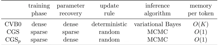
training parameter update inference memory phase recovery rule algorithm per token
CVB0 dense dense deterministic variational Bayes O(K) CGS sparse sparse random MCMC O(1) CGSp sparse dense random MCMC O(1)
Table 1: Properties of CVB0, CGS, and our proposed CGSp method.
the corresponding uncertainty information, as in CVB0, but within a Markov chain Monte Carlo framework, in order to draw on the benefits of both techniques. Our approach does not incur the memory overhead of CVB0, relative to CGS. The properties of CVB0, CGS, and our proposed estimators are summarized in Table 1.
It is important to note that we do not modify the CGS algorithm, and thus do not affect its runtime or memory requirements. Rather, we modify theprocedure for recovering parameter
estimates from collapsed Gibbs samples. After running the standard CGS algorithm (or a
modern accelerated approximate implementation) for a sufficient number of iterations, we obtain the standard document-topic and topic-word count matrices. At this point, instead of using the standard CGS parameter estimation equations to calculateθ andφ, we employ our proposed estimators. As a result, our estimators can be plugged in to the output of any CGS-based inference method, including modern variants of the algorithm such as Sparse LDA (Yao et al., 2009), Metropolis-Hastings-Walker (Li et al., 2014), LightLDA (Yuan et al., 2015), or WarpLDA (Chen et al., 2016), allowing for easy and wide adoption of our approach by the research community and in industry applications. Our algorithm is very simple to implement, requiring only slight modifications to existing CGS code. Popular LDA software packages such as MALLET (McCallum, 2002a) and Yahoo LDA (Smola and Narayanamurthy, 2010) could straightforwardly be extended to incorporate our methods, leading to improved parameter estimation in numerous practical topic modeling applications. In Section 5.7, we provide an application of our estimators to both MALLET’s Sparse LDA implementation, and to WarpLDA. When paired with a sparse CGS implementation, our approach gives the best of two worlds: making use of the full uncertainty information encoded in the dense Gibbs sampling transition probabilities in the final parameter recovery step, while still leveragingsparsity to accelerate the CGS training process.
In extensive experiments, we show that our approach leads to improved performance over standard CGS parameter estimators in both unsupervised and supervised LDA models. Our approach also outperforms the CVB0 algorithm under the majority of experimental conditions. The computational cost of our method is comparable that of a single (dense) CGS iteration, and we show that even when a state-of-the-art sparse implementation of the CGS training algorithm is used, this is a price well worth paying. Our results further illustrate the benefits of averaging over multiple samples for LDA parameter estimation. The contributions of our work can be summarized as follows:
• We present an extensive empirical comparison of our proposed estimators against those of standard CGS as well as the CVB0 algorithm (Asuncion et al., 2009) —a variant of the Collapsed Variational Bayesian inference (CVB) method—in both unsupervised and supervised learning settings, demonstrating the benefits of our approach.
• We provide an additional experimental comparison of the CGS and CVB0 algorithms regarding their convergence behavior, to further contextualize our empirical results.
Our theoretical and experimental results lead to three primary conclusions of interest to topic modeling practitioners:
• Averaging over multiple CGS samples to construct a point estimate for LDA parameters is beneficial to performance, in both the unsupervised and supervised settings, in cases where identifiability issues can be safely resolved.
• Using CVB0-style soft clustering to construct these point estimates is both valid and useful in an MCMC setting, and corresponds to implicitly averaging over many samples, thereby improving performance with little extra computational cost. This ports some of the benefits of CVB0’s use of dense uncertainty information to CGS, while retaining the sparsity advantages of that algorithm during training.
• Increasing the number of topics increases the benefit of our soft clustering/averaging approach over traditional CGS. While CVB0 outperforms CGS with few topics and a moderate number of iterations, CGS-based methods otherwise outperform CVB0, especially when using our improved estimators.
As this paper deals with LDA in both the unsupervised and the supervised setting, we will treat the following terms as equivalent when describing the procedure of learning an LDA model from training data: ‘estimation’, ‘fitting’, and ‘training’. Since we are in a Bayesian setting the word ‘inference’ will refer to the recovery of parameters, which are understood to be random variables, and/or the latent variables, and to the computation of the posterior distributions of parameters and latent variables. The term ‘prediction’ will be applied to the case of predicting on test data (i.e., data that was unobserved during training). Additionally, since Prior-LDA is essentially a special case of unsupervised LDA, we will focus our algorithm descriptions on the case of standard unsupervised LDA and specify the exceptions as they apply to Prior-LDA. Furthermore, we note here that we will be using the CGS algorithm described by Griffiths and Steyvers (2004), which approximates the LDA parameters of interest through iterative sampling in a Markov chain Monte Carlo (MCMC) procedure, unless otherwise specified.
2. Background and Related Work
In this section we provide the background necessary to describe our methods, and also establish the relevant notation.
2.1 Latent Dirichlet Allocation
LDA is a hierarchical Bayesian model that describes how a corpus of documents is generated via a set of unobserved topics. Each topic is parameterized by a discrete probability distribution over word types, which captures some coherent semantic theme within the corpus1. Here, we assume that this set of word types is the same for all topics (i.e., we have a single, shared vocabulary). Furthermore, LDA assumes that each document can be described as a discrete distribution over these topics. The process for generating each document then involves first sampling a topic from the document’s distribution over topics, and then sampling a word token from the corresponding topic’s distribution over word types. Formally, let us denote as V the size of the vocabulary (the set of unique word types) and asDT rain=|DT rain|andDT est=|DT est|the number of training and testing documents
respectively. We will useK to denote the number of topics. Similarly,v denotes a word type, wi a word token, ka topic (or in the case of Prior-LDA, a label), and zi a topic assignment.
The parameterφkv, k∈ {1...K}, v∈ {1...V}represents the probability of word typevunder
topic (or label)k, and θdk represents the probability of topic (or label) k for documentd.
Additionally αk will denote the parameter of the Dirichlet prior on θfor topic kand βv the
parameter of the Dirichlet prior onφfor word typev. Unless otherwise noted we assume for simplicity that the two priors are symmetric, so all the elements of the parameter vector α will have the same value (the same holds for the parameter vector β). The term Nddenotes
the number of word tokens in a given document d. Lastly, in the multi-label setting, Kd
stands for the set of labels that are associated with d. This notation is summarized in Table 2.
LDA assumes that a given corpus of documents has been generated as follows:
• For each topick∈ {1. . . K}, sample a discrete distribution φk over the word types of
the corpus from a Dirichlet(β).
• For each document d,
– Sample a discrete distributionθd over topics from a Dirichlet(α). – Sample a document lengthNd from a Poisson(ξ), with ξ∈R>0 – For each word tokenwi in document d,i∈ {1...Nd}:
∗ Sample a topiczi =kfrom discrete(θd). ∗ Sample a word typewi =v from discrete(φzi).
The goal of inference is to estimate the aforementioned θandφparameters—the discrete distributions for documents over topics, and topics over word types, respectively. In doing so, we learn a lower-dimensional representation of the structure of all documents in the corpus in terms of the topics. In the unsupervised learning context, this lower-dimensional
V the size of the vocabulary K the number of topics (or labels)
DT rain the number of training documents (similarly DT est) DT rain the set of training documents (similarly DT est)
d a document v a word type
wi a single word token, i.e., an instance of a word type wd the vector of word assignments in document d
k a topic (label)
zi the topic assignment to a word tokenwi
zd the vector of topic assignments to all word tokens of a document zdjk binary indicator variable, equals 1 IFF the jth word in document d
is assigned to topick Nd number of word tokens in d Kd set of topics (or labels) in d
nkv number of times that word type v has been assigned to topick across
the corpus
ndk number of word tokens in dthat have been assigned to topic k φk word type distribution for topic k
θd topic distribution for document d φkv topic-word type probability θdk document-topic probability
αk Dirichlet prior hyperparameter onθ for topic k βv Dirichlet prior hyperparameter onφ for word typev
γdik CVB0 variational probability of word tokenwi in documentdbeing
assigned to topic k
Table 2: Notation used throughout the article.
representation of documents is useful for both summarizing documents and for generating predictions about future, unobserved documents. In the supervised, multi-label learning context, extensions of the basic LDA model—such as Prior-LDA —put topics into one-to-one correspondence with labels, and the model is used for assigning labels to test documents.
2.2 Bayesian Inference, Prediction, and Parameter Estimation
LDA models are typically trained using Bayesian inference techniques. Given the observed training documents DT rain, the goal of Bayesian inference is to “invert” the assumed genera-tive process of the model, going “backwards” from the data to recover the parameters, by inferring the posterior distribution over them. In the case of LDA, the posterior distribution over parameters and latent variables is given by Bayes’ rule as
p(φ, θ,z|DT rain,α,β) =
p(DT rain|φ, θ,z)p(φ, θ,z|α,β) p(DT rain|α,β)
Being able to make use of the uncertainty encoded in the posterior distribution is a key benefit of the Bayesian approach. In the ideal procedure, having computed the posterior it can be used to make predictions on held-out data via the posterior predictive distribution, which computes the probability of new data by averaging over the parameters, weighted by their posterior probabilities. For a test documentw(new), under the LDA model we have
p(w(new)|DT rain,α,β) = Z Z
p(w(new)|φ, θ(new))p(θ(new)|α)dθ(new)p(φ|DT rain,α,β)dφ. Similarly, for supervised variants of LDA (discussed below), the ideal procedure is to average over all possible parameter values when predicting labels of new documents. In practice, however, it is intractable to compute or marginalize over the posterior, necessitating approximate inference techniques such as MCMC methods, which sample from the posterior using an appropriate Markov chain, and hence approximate it with the resulting set of samples. In particular, Nguyen et al. (2014) advocate using multiple samples to approximate the posterior, and averaging over the corresponding approximation to the posterior predictive distribution in order to make predictions for new data.
However, in the LDA literature it is much more common practice to simply approximate the posterior (and hence posterior predictive) distribution based on a single estimated value of the parameters (a point estimate). Although not ideal from a Bayesian perspective, a point estimate ˆφ, ˆθ of the parameters is convenient to work with as it is much easier for a human analyst to interpret, and is computationally much cheaper to use at test time when making predictions than using a collection of samples. In this paper, while strongly agreeing with the posterior predictive-based approach of Nguyen et al. (2014) in principle, we take the perspective that a point estimate is in many cases useful and desirable to have.
Following Nguyen et al. (2014), we do, however, have substantial reservations regarding the ubiquitous standard practice of using a single MCMC sample to obtain a point estimate. By interpreting MCMC as a “stochastic mode-finding algorithm” we can view this procedure as a poor-man’s approximation to the mode of the posterior. For many models, with a sufficiently large amount of data the posterior will approach a multivariate Gaussian under the Bernstein-von Mises theorem, and eventually become concentrated at a single point under certain general regularity conditions, cf. (Kass et al., 1990; Kleijn and van der Vaart, 2012). In this regime, a point estimate based on a single sample will in fact suffice. More generally, however, due to posterior uncertainty this procedure is unstable and consequently statistically inefficient: a parameter estimate from a posterior sample has an asymptotic relative efficiency (ARE) of 2, meaning, roughly speaking, that the variance of the estimator requires twice as many observations to match the variance of the ideal estimator, in the asymptotic Gaussian regime, under general regularity conditions, cf. (Wang et al., 2015).
As a compromise between the expensive full Bayesian posterior estimation procedure and noisy “stochastic mode-finding” with one sample, in this paper we propose to use the
posterior mean, approximated via multiple MCMC samples, as an estimator of choice in
Algorithm 1 Pseudocode for our proposed estimators. For simplicity, we consider only the case where a single CGS samplez is used.
function θp
Input: Burned-in CGS sample z with associated count matrices, documentsD ford= 1 to D do
ˆ
θd,p::=α|
for j= 1 to Nd do
v:=wdj . Retrieve the word token from the word position j in d.
fork= 1 to K do pdjk:= V nkv¬dj+βv
P
v0=1
(nkv0¬dj+βv0)
·(ndk¬dj +αk) .During testing, the first term is replaced byφkv
end for
pdj,::=pdj,:./ sum(pdj,:) . Normalize such thatPKk=1pdjk= 1,./denotes elementwise division. ˆ
θpd,::= ˆθd,p:+p|dv,: end for
ˆ
θd,p::= ˆθpd,:./sum(ˆθpd,:) . Normalize ˆθd,p:such thatPK k=1ˆθ
p dk= 1 end for
return θˆp end function
function φp
Input: Burned-in CGS sample z with associated count matrices, documentsDT rain fork= 1 to K do
ˆ
φpk,::=β| end for
ford= 1 to D do for j= 1 to Nd do
v:=wdj
fork= 1 to K do pdjk=
nkv¬dj+βv V
P
v0=1
(nkv0¬dj+βv0)
·(ndk¬dj+αk)
end for
pdj,::=pdj,:./ sum(pdj,:) .Normalize such thatPK
k=1pdjk= 1. ˆ
φp:,v := ˆφp:,v+pdj,: end for
end for
fork= 1 to K do ˆ
φpk:= ˆφpk,: ./sum( ˆφpk,:) . Normalize ˆφpk,:such thatPVv=1φˆpkv= 1
prefer this approach over an estimator based on a single sample. We expect a sample-based approximation to the posterior mean to be much more stable than an estimator based on a single sample, and our empirical results below will show that this is indeed the case in practice. In our proposed algorithm, we will show how to effectively average over multiple samples almost “for free”, based on samples and their Gibbs sampling transition probabilities. This is valuable in the very common setting where we are able to afford a moderate number of burn-in MCMC iterations, but we are not able to afford the much larger number of iterations to compute enough samples required to accurately estimate the posterior mean of the parameters.
It should be noted that averaging over MCMC samples for LDA, without care, can be invalidated due to a lack of identifiability. Multiple samples can each potentially encode different permutations of the topics, thereby destroying any correspondences between them, and Griffiths and Steyvers (2004) strongly warn against this. However, in this work, we will identify certain cases for which it is safe, and indeed highly beneficial, to average over samples in order to construct a point estimate, such as when estimating θat test time with the topics held fixed.
2.3 Collapsed Gibbs Sampling for LDA
The Collapsed Gibbs Sampling (CGS) algorithm for LDA, introduced by Griffiths and Steyvers (2004), marginalizes out the parametersφ and θ, and operates only on the latent variable assignmentsz. This leads to a simple but effective MCMC algorithm which mixes much more quickly than the naive Gibbs sampling algorithm. To compute the CGS updates efficiently, the algorithm maintains and makes use of several count matrices during sampling. We will employ the following notation for these count matrices: nkv represents the number
of times that word type vis assigned to topick across the corpus, andndk represents the
number of word tokens in documentdthat have been assigned to topic k. The notation for these count matrices is included in Table 2.
During sampling, CGS updates the hard assignment zi of a word token wi to one of
the topics k ∈ {1...K}. This update is performed sequentially for all word tokens in the corpus, for a fixed number of iterations. The update equation giving the probability of setting zi to topick, conditional onwi,d, the hyperparameters α andβ, and the current
topic assignments of all other word tokens (represented by·) is:
p(zi =k|wi =v, d,α,β,·)∝
nkv¬i+βv V
P v0=1
(nkv0¬i+βv0)
· ndk¬i+αk Nd+
K P k0=1
αk0
. (1)
In the above equation, one excludes from all count matrices the current topic assignment of wi, as indicated by the ¬inotation. A common practice is to run the Gibbs sampler for a
zi as well as for theθandφparameters. Samples are taken at a regular interval, often called
sampling lag.2
To compute point estimates for θ and φ, Rao-Blackwell estimators were employed in (Griffiths and Steyvers, 2004). Specifically, a point estimate of the probability of word type
v given topic kis computed as:
ˆ φkv =
nkv+βv V
P v0=1
(nkv0 +βv0)
. (2)
Similarly, a point estimate for the probability of the topic kgiven document dis given by:
ˆ θdk =
ndk+αk
Nd+ K P k0=1
αk0
. (3)
During prediction (i.e., when applying CGS on documents that were unobserved during training), a common practice is to fix theφ distributions and set them to the ones learned during estimation. The sampling update equation presented in Equation 1 thus becomes:
p(zi =k|wi =v, d,α,φ,ˆ ·)∝φˆkv·
ndk¬i+αk
Nd+ K P k0=1
αk0
. (4)
2.4 Labeled LDA
An extension to unsupervised LDA for supervised multi-label document classification was proposed by Ramage et al. (2009). Their algorithm, Labeled LDA (LLDA), employs a one-to-one correspondence between topics and labels. During estimation of the model, the possible assignments for a word token to a topic are constrained to the training document’s observed labels. Therefore, during training, the sampling update of Equation 1, becomes:
p(zi=k|wi=v, d,α,β,·)∝
nkv¬i+βv V
P
v0=1
(nkv0¬i+βv0)
· ndk¬i+αk
Nd+ K
P
k0=1
αk0
, ifk∈ Kd
0, otherwise.
(5)
Inference on test documents is performed similarly to standard LDA; estimates of the label–word types distributions,φ, are learned on the training data and are fixed, and then the test documents’θ distributions are estimated using Equation 3. Unlike in unsupervised LDA, where topics can change from iteration to iteration (the label switching problem), in LLDA topics remain steady (anchored to a label) and therefore it is possible to average point estimates ofφ andθ over multiple Markov chains, thereby improving performance.
Ramage et al. (2011) have introduced PLDA to relax the constraints of LLDA and exploit the unsupervised and supervised forms of LDA simultaneously. Their algorithm attempts to model hidden topics within each label, as well as unlabeled, corpus-wide latent topics.
Rubin et al. (2012) presented two extensions of the LLDA model. The first one, Prior-LDA, takes into account the label frequencies in the corpus via an informative Dirichlet prior over parameter θ (we describe this process in detail in Section 6.3). The second extension, Dependency LDA, takes into account label dependencies by following a two stage approach: first, an unsupervised LDA model is trained on the observed labels. The estimated θ0 parameters incorporate information about the label dependencies. Second, the LLDA model is trained as described in the previous paragraph. During prediction, the previously estimatedθ0 parameters of the unsupervised LDA model are used to calculate an asymmetrical hyperparameter αdk, which is in turn used to compute theθ parameters of
the LLDA model.
2.5 Collapsed Variational Bayes with Zero Order Information – CVB0
Collapsed Variational Bayesian (CVB) inference (Teh et al., 2006) is a deterministic inference technique for LDA. The key idea is to improve on Variational Bayes (VB) by marginalizing out θandφas in a collapsed Gibbs sampler. The key parameters in CVB are theγdi variational
distributions over the topics, with γdik representing the probability of the assignment of
topic k to the word token wi in document d, under the variational distribution. As the
exact implementation of CVB is computationally expensive, the authors propose a second-order Taylor expansion as an approximation to compute the parameters of interest, which nevertheless improves over VB inference with respect to prediction performance.
Asuncion et al. (2009) presented a further approximation for CVB, by using a zero order Taylor expansion approximation.3 The update equation for CVB0 is given by:
γdik ∝ n0kw
i¬i+βwi
V P v0=1
(n0kv0¬i+βv0)
(n0dk¬i+αk) (6)
with n0kv=
D P d=1
P
j:wdj=vγdjk,n 0
dk = PNd
j=1γdjk.
Point estimates for θandφare retrieved from the same equations as in CGS (Equations 2 and 3). Even though the above update equation looks very similar to the one for CGS, the two algorithms have a couple of key differences. First, the counts n0kv andn0dk for CVB0 differ from the respective ones for CGS; the former are summations over the variational probabilities while the latter sum over the topic assignmentszi of topics to words. Second,
CVB0 differs from CGS in that in every pass, instead of probabilistically sampling a hard topic-assignment for every token based on the sampling distribution in Equation 1, it keeps (and updates) that probability distribution for every word token. A consequence of this procedure is that CVB0 is a deterministic algorithm, whereas CGS is a stochastic algorithm (Asuncion, 2010). The deterministic nature of CVB0 allows it to converge faster than other
inference techniques.
On the other hand, the CVB0 algorithm has significantly larger memory requirements as it needs to store the variational distribution γ for every token in the corpus. More recently, a stochastic extension of CVB0, SCVB0, was presented by Foulds et al. (2013), inspired by
the Stochastic Variational Bayes (SVB) algorithm of Hoffman et al. (2010a). Both SCVB0 and SVB focus on efficient and fast inference of the LDA parameters in massive-scale data scenarios. SCVB0 also improves the memory requirements of CVB0. Since CVB0 maintains full, dense probability distributions for each word token, it is unable to leverage sparsity to accelerate the algorithm, unlike CGS (Yao et al., 2009; Li et al., 2014; Yuan et al., 2015; Chen et al., 2016). Inspired by CVB0, in our work we aim to leverage the full distributional uncertainty information per word token, in the context of the parameter estimation step of the CGS algorithm, while maintaining the valuable sparsity properties of that algorithm during the training process.
3. CGSp for Document-Topic Parameter Estimation
In this section we present our new estimator for the document-topic (θd) parameters of
LDA that make use of the full distributions of word tokens over topics. For simplicity, we first describe the case ofθd estimation during prediction and then extend our theory toθd
estimation during training. We present our estimator for the topic-word parameters (φk) in
the following section.
3.1 Standard CGS θd Estimator
The standard estimator for document d’s parametersθd from a collapsed Gibbs samplezd
(Equation 3), due to Griffiths and Steyvers (2004), corresponds to the posterior predictive distribution over topic assignments, i.e.,
ˆ
θdk ,p(z(new)=k|zd,α) (7)
= Z
p(z(new)=k, θd|zd,α) dθd (8)
= Z
p(z(new)=k|θd)p(θd|zd,α) dθd (9)
= Z
θdkp(θd|zd,α) dθd (10)
=Ep(θd|zd,α)[θdk] (11)
=EDirichlet(θd|α+nd)[θdk] (12)
= ndk+αk Nd+PKk0=1αk0
where the last two lines follow from Dirichlet/multinomial conjugacy, and from the mean of a Dirichlet distribution, respectively. Here, z(new) corresponds to a hypothetical “new” word in the document. The posterior predictive distribution can be understood via the urn process interpretation of collapsed Dirichlet-multinomial models. After marginalizing out the parametersθ of a multinomial distributionx∼Multinomial(θ, N) with a Dirichlet prior θ∼Dirichlet(α), we arrive at an urn process called the Dirichlet-multinomial distribution, a.k.a. the multivariate Polya urn, cf. (Minka, 2000). The urn process is as follows:
• Begin with an empty urn
• For eachk, 1≤k≤K
– add αk balls of colork to the urn
• For eachi, 1≤i≤N
– Reach into the urn and draw a ball uniformly at random
– Observe its color,k. Count it, i.e., add one toxk
– Place the ball back in the urn, along with anew ball of the same color.
We can interpret the posterior predictive distribution above as the probability of the next ball in the urn, i.e., the next word in the document, if we were to add one more word, by reaching into the urn once more.
3.2 A Marginalized Estimation Principle
The topic assignment vectorzd for test documentdis a latent variable which typically has
quite substantial posterior uncertainty associated with it, and yet the most common practice is to ignore this uncertainty and construct a point estimate ofθdfrom a single zd sample,
which can be detrimental to performance (Nguyen et al., 2014). Following Griffiths and Steyvers (2004), we assume that the predictive probability of a new word’s topic assignment z(new) is a principled estimate of θd. Differently to previous work, though, we take the
perspective that the latent zd is a nuisance variable which should be marginalized out. This
leads to a marginalized version of Griffiths and Steyvers’ estimator,
¯
θdk ,p(z(new)=k|wd, φ,α) = X
zd
p(z(new) =k,zd|wd, φ,α) . (14)
Due to its treatment of uncertainty inzd, we advocate for ¯θdas a gold standard principle for
constructing a point estimate ofθd. We will introduce computationally efficient Monte Carlo
procedures for making predictions by approximating the posterior predictive distribution. They do not aim to compute a point estimate from multiple samples, however their Single
Average prediction strategy can be seen to be equivalent to using a naive Monte Carlo
estimate (given in Equation 26) of Equation 14 in the context of predicting held-out words.
3.2.1 Interpretations
We can interpret the estimator from Equation 14 in several other ways.
Expected Griffiths and Steyvers estimator: The estimator ¯θdcan readily be seen to
be the posterior mean of the Griffiths and Steyvers estimator ˆθd:
¯
θdk=p(z(new) =k|wd, φ,α) = X
zd
p(z(new)=k,zd|wd, φ,α) (15)
=X
zd
p(z(new)=k|zd,α)p(zd|wd, φ,α) (16)
=Ep(zd|wd,φ,α)[p(z
(new)=k|z
d,α)] (17)
=Ep(zd|wd,φ,α)[ˆθdk] . (18)
Posterior mean of θd: Griffiths and Steyvers’ estimator can be viewed as the posterior
mean ofθd, given zd (Equation 11). Along these lines, we can interpret ¯θd as the marginal
posterior mean:
¯
θdk =p(z(new)=k|wd, φ,α) =Ep(zd|wd,φ,α)[ˆθdk] (19)
=Ep(zd|wd,φ,α)
h
Ep(θd|zd,α)[θdk]
i
(20)
=Ep(θd|wd,φ,α)[θdk] , (21)
where the last line follows by the law of total expectation.
Urn model interpretation: To interpret the estimator from an urn model perspective, we can plug in Equation 13:
¯
θdk=p(z(new) =k|wd, φ,α) = X
zd
p(z(new)=k|zd,α)p(zd|wd, φ,α) (22)
=X
zd
ndk+αk Nd+PKk0=1αk0
p(zd|wd, φ,α) . (23)
We can view this as a mixture of urn models. It can be simulated by picking an urn with colored balls in it corresponding to the count vectornd+α, with probability according to the
posterior p(zd|wd, φ,α), then selecting a colored ball, corresponding to a topic assignment,
from this urn uniformly at random. Alternatively, we can model this equation with a single urn, with (fractional) colored balls placed in it according to the count vector,
¯ θdk ∝
X
zd
(ndk+αk)p(zd|wd, φ,α) = X
zd
p(zd|wd, φ,α)ndk+αk , (24)
3.2.2 Monte Carlo algorithms for computing the estimator
Due to the intractable sum overzd, we cannot compute ¯θd exactly. A straightforward Monte
Carlo estimate of ¯θd is given by
¯
θdk=Ep(zd|wd,φ,α)[p(z
(new)=k|z
d,α)] =Ep(zd|wd,φ,α)
h ndk+αk Nd+
PK k0=1αk0
i (25) ≈ 1 S S X i=1
n(dki)+αk Nd+
PK k0=1αk0
, (26)
where each of the count variables n(di) corresponds to a sample zd(i) ∼p(zd|wd, φ,α).
Algo-rithmically, this corresponds to drawing multiple MCMC samples of zd and averaging the
Griffiths and Steyvers estimator ˆθd over them. Alternatively, by linearity of expectation we
can shift the expectation inwards to rewrite the above as
Ep(zd|wd,φ,α)
h ndk+αk Nd+PKk0=1αk0
i
=Ep(zd|wd,φ,α)
h PNd
j=1zdjk+αk Nd+PKk0=1αk0 i
(27)
= PNd
j=1Ep(zd|wd,φ,α)[zdjk] +αk
Nd+ PK
k0=1αk0
. (28)
This leads to another Monte Carlo estimate,
¯ θdk ≈
PNd
j=1 1 S
PS i=1z
(i) djk+αk Nd+PKk0=1αk0
. (29)
In this case we would once again draw multiple MCMC samples of zd, but average over
the samples to compute the proportion of times that each word is assigned to each topic, applying Griffiths and Steyvers’ estimator to the resulting expected total counts. It can straightforwardly be shown that this estimator is mathematically equivalent to the estimator of Equation 26, so this algorithm will perform identically to that method. We mention this formulation for expository purposes, as it will be used as a launching point for deriving our proposed CGSp algorithm.
3.3 CGSp for θd
We aim to design a statistically and computationally efficient Monte Carlo algorithm which improves on the above algorithms. To do this, we first consider a hypothetical Monte Carlo algorithm which is more expensive but easily understood, using Equation 29 as a starting point. We then propose our algorithm, CGSp, as a more computationally efficient version
of this hypothetical method. Let z(di) ∼p(zd|wd, φ,α), i∈ {1, . . . , S} be S samples from
We can therefore estimate posterior expectations of any quantity of interest using these samples instead of thez(di)’s, and in particular:
¯ θdk ≈
PNd
j=1 SL1 PS
i=1 PL
l=1z (i,l)→j djk +αk Nd+
PK k0=1αk0
. (30)
This method increases the sample size, and also the effective sample size, relative to the method of Equation 29, but also greatly increases the computational effort to obtain the Monte Carlo estimator, making it relatively impractical. Fortunately, a variant of this procedure exists which is both computationally faster and has lower variance. Let T(z(di)→j|z(di), φ) be the transition operator for a Gibbs update on the jth topic assignment. Holding the other assignmentsz(di¬)j fixed, we have the partially collapsed Gibbs update
T(z(djki)→j = 1|z(di), φ)∝φkwd,j
n(dki)¬j+αk Nd¬j+PKk0=1αk0
. (31)
By the strong law of large numbers,
1 L
L X
l=1
zdjk(i,l)→j →E
T(z(di)→j|z(di),φ)[z (i)→j
djk ] =T(z (i)→j djk |z
(i)
d , φ) as L→ ∞ with probability 1.
(32)
So for the cost of a single Gibbs sweep through the document, we can obtain an effective number of inner loop samplesL=∞ by plugging in the Gibbs sampling probabilities as the expected topic counts in Equation 30. This leads to our proposed estimator for θdk:
ˆ θdkp ,
PNd
j=1 1 S
PS i=1T(z
(i)→j djk |z
(i)
d , φ) +αk Nd+PKk0=1αk0
. (33)
This method is equivalent to averaging over an infinite number of Gibbs samples adjacent to our initial samplesi= 1, . . . , Sin order to estimate each word’s topic assignment probabilities, and thereby estimate the expected topic counts for the document, which correspond to our estimate ofθd. By the Rao-Blackwell theorem, it has lower variance than the method in
Equation 30 with finite L. We refer to this Monte Carlo procedure as CGSp, for collapsed
Gibbs sampling with probabilities maintained.
ˆ θdkp ∝
Nd X j=1 1 S S X i=1
T(zdjk(i)→j|z(di), φ) +αk (34)
= Nd X j=1 1 S S X i=1
ET(z(i)→j
d |z
(i)
d ,φ)
[z(djki)→j] +αk (35)
≈ Nd
X
j=1
Ep(zd|wd,φ,α)
h ET(z→j
d |zd,φ)[z →j djk]
i
+αk (36)
=
Nd
X
j=1 Ep(z→j
d |wd,φ,α)[z →j
djk] +αk (by the law of total expectation)
=
Nd
X
j=1
Ep(zd|wd,φ,α)[zdjk] +αk (by stationarity of the Gibbs sampler)
=Ep(zd|wd,φ,α)[
Nd
X
j=1
zdjk] +αk (37)
=Ep(zd|wd,φ,α)[ndk+αk] (38)
∝Ep(zd|wd,φ,α)[
ndk+αk Nd+PKk0=1αk0
] (39)
=p(z(new)=k|wd, φ,α) . (by Equation 25)
We advocate the use of this procedure even when we can only afford a single burned-in sample, i.e.,S = 1, as a cheap approximation top(z(new) =k|wd, φ,α) which can be used as a plug-in
replacement to Griffiths and Steyvers (2004)’s single sample estimator p(z(new)=k|zd,α).
Indeed, the increased stability of our estimator, due to implicit averaging, is expected to be especially valuable whenS = 1. We emphasize three primary observations arising from the above analysis.
(1) We have shown that it is valid and potentially beneficial to use “soft” probabilistic counts instead of hard assignment counts when computing parameter estimates from collapsed Gibbs samples. This ports the soft clustering methodology of CVB0 to the CGS setting at estimation time. While our approach computes soft counts via Gibbs sampling transition probabilities and CVB0 uses variational distributions, the corresponding equations to compute them are very similar, cf. Equations 1, 4, and 6.
(2) Averaging these (hard or soft) count matrices over multiple samples can be performed to improve the stability of the estimators, as long as identifiability is resolved, e.g., at test time with the topics held fixed.
This last point is crucial in many common practical applications of topic modeling where we have a limited computational budget per document at prediction time, and can afford only a modest burn-in period, and few samples after burn-in. This situation frequently arises when evaluating topic models, for which a novel approach is typically compared to multiple baseline methods on a test set containing up to tens of thousands of documents, with the entire experiment being repeated across multiple corpora and/or training folds. The computational challenge is greatly exacerbated when evaluating topic model training algorithms, for which the above must be repeated at many stages of the training process (Foulds and Smyth, 2014). For instance, Asuncion et al. (2009) state that “in our experiments we don’t perform averaging over samples for CGS . . . [in part] for computational reasons.” Computational efficiency at test time is also essential when using topic modeling for multi-label document classification (Ramage et al., 2009, 2011; Rubin et al., 2012), for which a deployed system may need to perform inference on a never-ending stream of incoming test documents.
Pseudocode illustrating the proposed method is provided in Algorithm 1. It should be noted than any existing CGS implementation can very straightforwardly be modified to apply our proposed technique, including MALLET (McCallum, 2002a), Yahoo LDA (Smola and Narayanamurthy, 2010), and WarpLDA (Chen et al., 2016). Our method is compatible with modern sparse and parallel implementations of CGS, as the final estimation procedure does not need to alter the training process. This can lead to a “best of both worlds” situation, where sparsity is leveraged during the expensive CGS inference process, but the full dense distributions are used during the relatively inexpensive parameter recovery step, which in many topic modeling applications is performed only once. In this setting, the improved performance is typically worth the computational overhead (which is similar to that of a single dense CGS update), as we demonstrate in Section 5.8. A practical implementation of our estimators can further leverage the fact that the count matrices are not modified during the procedure, by computing the sampling distribution only once for each distinct word type in each document, and by performing the computations in parallel. In the following we will sometimes abuse notation and denote the procedure of using ˆθpd to estimate the θd’s as θp
(and similarly for the procedure to estimate φ, denoted φp, introduced below).
3.3.1 CGSp for estimating θd for training documents
During the training phase, we can apply the same procedure to estimate θd for training
documents based on a given collapsed Gibbs sample z(i):
ˆ θdkp =
PNd
j=1T(z (i)→j
djk |z(i), φ) +αk Nd+PKk0=1αk0
. (40)
The collapsed Gibbs sampler does not explicitly maintain an estimate of φto plug into the above. However, the Griffiths and Steyvers estimator forφ(Equation 2) can be obtained from the same count matrices that CGS computes, as it corresponds almost exactly to the first term on the right hand side of Equation 1. Alternatively, below we propose a novel estimator for φwhich can also be used here with a little bit more computational effort.
identifiability of the topics, which can potentially be problematic (Griffiths and Steyvers, 2004). We do not consider this procedure further here. It is however safe to apply Equation 33 to multiple MCMC samples forzdthat are generated while holding φ fixed, i.e., treating
documentdas a test document for the purposes of estimatingθd given the ˆφfrom z(i). 4. CGSp for Topic - Word Types Parameter Estimation
By applying the same approach as forθp, plugging in Gibbs transition probabilities instead of indicator variables into Equation 2, we arrive at an analogous technique for estimatingφ:
ˆ φpkv =
PDT rain
d=1 P
j:wd,j=vT(z
(i)→j djk |z
(i)) +β v
PDT rain
d=1
PNd
j=1T(z (i)→j
djk |z(i)) + PV
v0=1βv0
, (41)
where T(z(d,ji)→j|z(i)) corresponds to the collapsed Gibbs update in Equation 1. While the intuition of the above method is clear, there are several technical complications to an analogous derivation for it. Nevertheless, we show that the same reasoning essentially holds for φ, with minor approximations. In the following, we outline a justification for the φp estimator, with emphasis on the places where the argument fromθp does not apply, along with well-principled approximation steps to resolve these differences.
First, consider the estimation principle underlying the technique. For topics φ, the standard Rao-Blackwellized estimator of Griffiths and Steyvers (2004), given by Equation 2, once again corresponds to the posterior predictive distribution,
ˆ
φkv ,p(w(new)=v|z,w,β, z(new)=k)
= Z
p(w(new)=v, φk|z,w,β, z(new)=k)dφk
= Z
p(w(new)=v|φk, z(new)=k)p(φk|wz=k,β)dφk
=EDirichlet(nk+β)[φkv]
= nkv+βv
V P v0=1
(nv0k+βv0)
, (42)
where wz=k is the collection of word tokens assigned to topic k. This estimator again
conditions on the latent variable assignments z, which are uncertain quantities. We desire a marginalized estimator, summing out the latent variablesz. However, without conditioning on z, the topic index kloses its meaning because the topics are not identifiable. The naive marginalized estimator
¯
φkv ,p(w(new)=v|w,β, z(new)=k) = X
z
p(w(new) =v,z|w,β, z(new)=k) (43)
for all values of z considered. Suppose, by some oracle, we know that z belongs to some
identified subset of assignments ˙Z, for which topic indices are aligned between all elements z0 ∈Z˙. We are then able to properly define our idealized estimator with respect to ˙Z,
¯
φ( ˙kvZ),p(w(new) =v|w,β, z(new)=k,z∈Z˙) =X
z∈Z˙
p(w(new)=v,z|w,β, z(new)=k,z∈Z˙) . (44) Regarding our proposed technique, the Monte Carlo estimator in Equation 41 implicitly averages over the set of possible Gibbs samples ZGibbs(z(i)) that are adjacent to sample z(i), i.e., the candidate z assignments that differ from z(i) in a single entry. A difference of a single word is extremely unlikely to cause label switching for a realistic corpus, so the topics will almost certainly be aligned for each of the adjacent Gibbs samples that the estimator implicitly averages over. The empirical results of Nguyen et al. (2014) also support this, as they found that averaging over multiple samples from the same MCMC chain was beneficial to performance, which suggests that identifiability was not a problem even for MCMC samples that are many iterations apart. Hence, we take ¯φ(ZGibbs(z(i)))
kv as
our idealized estimator, under the supposition that ZGibbs(z(i)) is identified, and we aim to
derive Equation 41 as a Monte Carlo algorithm that efficiently approximates it. To accomplish this, following the derivation for ˆθp, we would like to show that
(1) we can use a Monte Carlo estimator in which thezd,j’s can be sampled individually,
as in Equation 29, and
(2) the transition probabilities in Equation 41 can be used to implement this estimator with an effectively infinite number of adjacent Gibbs samples, as in Section 3.3.
While the previous stationarity argument for (2) still applies, there is a further complication for (1). For ˆθp, linearity of expectation was sufficient to show in Equation 28 that
Ep(zd|wd,φ,α)
h PNd
j=1zdjk+αk Nd+PKk0=1αk0 i
= PNd
j=1Ep(zd|wd,φ,α)[zdjk] +αk
Nd+PKk0=1αk0
.
We cannot use this argument directly for ˆφp because in this case the denominator of the Griffiths and Stevyers estimator, which is averaged over, also includes z terms which are involved in the expectation:
¯
φ(ZGibbs(z(i)))
kv =Ep(z|w,β,z∈ZGibbs(z(i)))
h
PDT rain
d=1 P
j:wd,j=vzdjk+βv
PDT rain
d=1
PNd
j=1zdjk+PVv0=1βv0 i
. (45)
The issue here is that the adjacent Gibbs samples modify the overall counts per topic nk,
PDT rain
d=1
PNd
j=1zdjk. However, between adjacent Gibbs samples zand z(i), the corresponding topic countsnk are within±1 of n
(i)
impact of a single word is negigible, i.e.,
DT rain
X
d=1 Nd
X
j=1 zdjk∈
nDXT rain
d=1 Nd
X
j=1 zdjk(i),
DT rain
X
d=1 Nd
X
j=1
z(djki) ±1o≈ DT rain
X
d=1 Nd
X
j=1 z(djki) ,
forz∈ZGibbs(z(i)) , DT rain
X
d=1 Nd
X
j=1
zdjk>>1 . (46)
In this case, we see from Equation 46 that for a corpus in whichnk >>1, for all practical
purposes the denominator in Equation 45 is essentially constant over all adjacent Gibbs samples, and so (1) still holds approximately, and we have
¯
φ(ZGibbs(z(i)))
kv =Ep(z|w,β,z∈ZGibbs(z(i)))
h
PDT rain
d=1 P
j:wd,j=vzdjk+βv
PDT rain
d=1
PNd
j=1zdjk+PVv0=1βv0 i
≈Ep(z|w,β,z∈ZGibbs(z(i)))
h
PDT rain
d=1 P
j:wd,j=vzdjk+βv
PDT rain
d=1
PNd
j=1z (i) djk+
PV v0=1βv0
i
=
PDT rain
d=1 P
j:wd,j=vEp(z|w,β,z∈ZGibbs(z(i)))[zdjk] +βv
PDT rain
d=1
PNd
j=1z (i) djk+
PV v0=1βv0
. (47)
A related argument was also made by Asuncion et al. (2009), who note that several topic modeling inference algorithms differ only by offsets of 1 or 0.5 to the counts, and state that “since nk is usually large, we do not expect [a small offset] to play a large role in learning.”
To formalize this intuition, as we show in Appendix B, the approximation can be bounded from below and from above as a function ofn(ki) as:
n(ki)+PV v0=1βv0 n(ki)+PV
v0=1βv0+ 1
Ep(z|w,β,z∈Z
Gibbs(z(i)))
h
PDT rain
d=1 P
j:wd,j=vzdjk+βv
PDT rain
d=1
PNd
j=1z (i) djk+
PV v0=1βv0
i
≤Ep(z|w,β,z∈Z
Gibbs(z(i)))
h
PDT rain
d=1 P
j:wd,j=vzdjk+βv
PDT rain
d=1
PNd
j=1zdjk+PVv0=1βv0 i
≤ n
(i) k +
PV v0=1βv0 n(ki)+PV
v0=1βv0−1
Ep(z|w,β,z∈Z
Gibbs(z(i)))
h
PDT rain
d=1 P
j:wd,j=vzdjk+βv
PDT rain
d=1
PNd j=1z
(i) djk+
PV v0=1βv0
i
, (48)
forn(ki)>0. Since lim
n(ki)→∞
n(ki)+PV v0=1βv0
n(ki)+PV
v0=1βv0+1
= 1 and lim
n(ki)→∞
n(ki)+PV v0=1βv0
n(ki)+PV
v0=1βv0−1
= 1, the left
and right hand sides of Equation 47 will converge in the limit as then(ki)’s go to infinity, e.g., when increasing the counts via a stream of incoming documents. In Appendix C, we provide a further empirical illustration of this approximation, by taking subsets of the documents in the corpus to varynk, and observing that as nk increases the difference between the left
Finally, using the same stationarity and law of large numbers arguments as before, we obtain the ˆφp estimator by plugging in the transition operator, and then renormalizing,
ˆ φpkv ∝
DT rain
X
d=1 X
j:wd,j=v
Ep(z|w,β,z∈Z
Gibbs(z(i)))[zdjk] +βv =
DT rain
X
d=1 X
j:wd,j=v
T(zdjk(i)→j|z(i)) +βv .
(49)
More formally, the full argument is given mathematically as
ˆ φpkv∝
DT rain
X
d=1 X
j:wd,j=v
T(z(djki)→j|z(i)) +βv (50)
=
DT rain
X
d=1 X
j:wdj=v
ET(z(i)→j
d |z
(i)
d )
[z(djki)→j] +βv (51)
=
DT rain
X
d=1 X
j:wdj=v
Ep(z|w,β,z∈Z
Gibbs(z(i)))[zdjk] +βv
(by stationarity of the Gibbs sampler)
∝
PDT rain
d=1 P
j:wdj=vEp(z|w,β,z∈ZGibbs(z(i)))[zdjk] +βv
PDT rain
d=1
PNd
j=1z (i) djk+
PV v0=1βv0
(52)
=Ep(z|w,β,z∈Z
Gibbs(z(i)))
h
PDT rain
d=1 P
j:wdj=vzdjk+βv
PDT rain
d=1
PNd
j=1z (i) djk+
PV v0=1βv0
i
(53)
≈Ep(z|w,β,z∈Z
Gibbs(z(i)))
h
PDT rain
d=1 P
j:wdj=vzdjk+βv
PDT rain
d=1
PNd
j=1zdjk+PVv0=1βv0 i
(ifnk>>1)
=p(w(new) =v|w,β, z(new)=k,z∈ZGibbs(z(i))) . (54)
In Algorithm 1, along with θp’s procedure, we also present the pseudocode for the φp estimator.
5. Unsupervised Learning Experiments—LDA
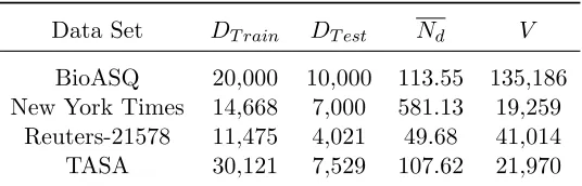
Data Set DT rain DT est Nd V
BioASQ 20,000 10,000 113.55 135,186 New York Times 14,668 7,000 581.13 19,259
Reuters-21578 11,475 4,021 49.68 41,014 TASA 30,121 7,529 107.62 21,970
Table 3: Statistics for the data sets used in the unsupervised learning experiments. Average document length and number of word types refer to the training sets.
5.1 Data Sets
Four data sets were used in the unsupervised setting: a) BioASQ, b) New York Times, c) Reuters-21578 and d) TASA. The number of documents in the training and test sets, the average length of the training documents and the size of the vocabulary of word types found in the training set are presented in Table 3.
The first data set originates from the BioASQ challenge (Balikas et al., 2014) that deals with large-scale online multi-label classification of biomedical journal articles. This learning task is particularly challenging as the taxonomy of labels includes around 27,000 terms, with highly imbalanced frequencies. For the unsupervised experiments of this section, we used the 30,000 last documents of the BioASQ corpus of the year 2014, using the first 20,000 as training documents and the rest as test documents. To construct the data set we concatenated the abstract and title of each article and removed common stopwords. The remaining unigrams were used as word types.
The second data set contains articles published by the New York Times, manually annotated via their indexing service. We used the same data set as used by Rubin et al. (2012), with the same training set (14,668 documents) and keeping the first 7,000 documents
for testing (out of the 15,989 of the original paper).
The third data set4 contains documents from the Reutersnews-wire and has been widely used among researchers for almost two decades. The split that we used has 11,475 documents for training and 4,021 documents for testing. We preprocessed the corpus by removing common stopwords.
The TASAdata set contains 37,650 documents of diverse educational materials (e.g., health, sciences, etc) collected by Touchstone Applied Science Associates (Landauer et al., 1998). We used the first 30,121 documents as a training set and the remaining as a test set. The corpus already had stopwords and infrequent words removed, so we did not perform any further preprocessing.
5.2 Evaluation
Evaluation of LDA models typically focuses on the probability of a set of held-out documents given an already trained model (Wallach et al., 2009). In this context, one must compute the model’s posterior predictive likelihood of all words in the test set, given estimates of the topic parameters φand the document-level mixture parameters θ.
The log likelihood of a set of test documents DT est, given an already estimated model M, is given by Heinrich (2004) as:
Log Likelihood =
DT est
X
d=1
logp(wd|M) = DT est
X
d=1 Nd
X
i=1 log
K X
k=1
(φkv·θdk) (55)
with wi =v. The perplexity will be:
Perplexity = exp(−Log Likelihood DT est
P d=1
Nd
) (56)
where lower values of perplexity signify a better model.
Sinceθdis unknown for test documents, and is intractable to marginalize over, a common
practice in the literature in order to compute the above likelihood is to run the CGS algorithm for a few iterations on the first half of each document, and then to compute the perplexity of the held-out data (the second half of each document), based on the trained model’s posterior predictive distribution over words (Asuncion et al., 2009). This is the approach we follow.
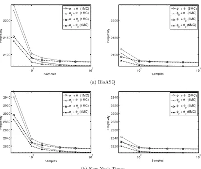
5.3 Comparison between CGS and CGSp
In this first experiment, the motivation is to validate the previously presented theory behind theφp and θp methods. Specifically, we are interested in verifying the following hypothesis:
given a single burned-in sample, ˆφp or ˆθp will more effectively estimate the respective LDA
parameters compared to the standard estimators, since the CGSp estimators make use of
the full dense probabilities, through the infinite l-steps of Eq. 33. This advantage would correspond to lower perplexity values for a single burned-in sample for the CGSp estimators
compared to the standard CGS estimator. Furthermore, when averaging over multiple samples to estimate theθparameters during prediction, we expect that the θp and standard θ estimators will eventually converge to the same solution given enough samples or Markov chains, since θp aims to compute the posterior mean. However, we expect that θp will converge to the posterior mean more rapidly in the number of samples that are averaged over than the standard estimator θ, with correspondingly faster improvement in perplexity.
For this experiment we used all four data sets and considered four different topic number configurations (20, 50, 100, 500). For brevity, we report only the results for K= 100 and include the rest of the plots in Appendix D. During training, we ran one Markov chain for 200 iterations and took a single sample to calculate φ and φp from the same chain.
During prediction, sinceφis fixed and topics are not exchanged through the Gibbs sampler’s iterations, we took multiple samples from multiple Markov chains, and averaged over these samples using theθ (standard CGS) andθp estimators. The burn-in period for the Gibbs
sampler was set to 50 iterations and a sampling lag of 5 iterations was used. The α and β hyperparameters were symmetrical across all topics and words respectively and set such that αk= 0.1 andβv = 0.01. Finally, to ensure fairness between theθandθp estimators, we
used the same samples from the same chains to compute the respective estimates.
combinations of the estimators are depicted. By observing the results we notice some key points across all plots. First, if we consider the case where only one burned-in sample is used, corresponding to the left-most points in the plots, we can notice that bothθp methods (φ+θp and φp +θp) decisively outperform the other two methods. This observation is particularly important for scenarios where we can’t afford to average over many samples due to computational or time limitations, as frequently occurs during the comparative evaluation of topic modeling methods, and in multi-label document classification.
We also see that the φp methods (φp+θandφp+θp) have a short but steady advantage over the respective φ estimators. This advantage is not diminished for more samples or Markov chains, suggesting thatφp is actually a more accurate estimator thanφ. We also remind here that in unsupervised scenarios we cannot average over samples to compute a φestimate during training, since topics may be interchanged between iterations. A third remark, also aligned with our theoretical results, is that θ and θp converge to the same solution after a sufficient number of samples are averaged over, although θp converges much more rapidly. Overall, these findings confirm that indeed bothθp andφp constitute improved estimators compared to the respective standard ones: θp provides more rapid convergence than using the standard estimator θ when averaging over samples for prediction on test documents, andφp improves perplexity due to implicit averaging. The rest of the plots in Appendix D are in accordance with the above observations.
5.4 Word Association: φp vs φ
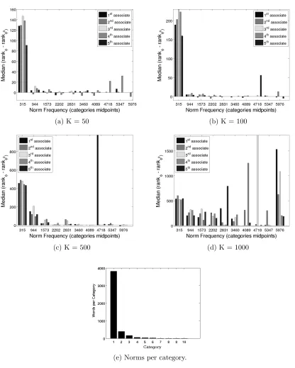
In this experiment, we compareφp with φon a word association task. In word association, a given word, called the norm or cue word, is associated with a number of semantically related words, calledtargets orassociates. We consider the data set provided by Nelson et al. (2004), which contains a set of 5,019 norm words and for each of them a set of associate words provided by human annotators. We aim to see how, given a specific cue word, the two LDA estimators rank the corresponding associates, in order to assess which of the two performs better at predicting the targets, in terms of the median difference in ranks. The word association task provides a useful benchmark for evaluating the extent to which the topic representations are a good model of human semantic representation (Griffiths et al., 2007).
(a) BioASQ
(b) New York Times
Figure 1: Perplexity against the number of samples averaged over, for the CGSp estimators
and standard CGS. Results are taken by averaging over 5 different runs. Samples are taken after a burn-in period of 50 iterations.
cue word and w2 denotes each of the rest of the vocabulary word types. Supposing thatw1 and w2 belong to the same topicz, and assuming a uniform prior on z, we have5
p(w2|w1) = X
z
p(w2|z)p(z|w1) = X
z
p(w2|z)
p(w1|z)p(z) P
z0
p(w1|z0)p(z0) =X
z
p(w2|z)
p(w1|z) P
z0
p(w1|z0) . (57)
Next, we consider the first five associate words of the norm w1 and obtain the rank for each of them according to the probabilitiesp(w2|w1), for each ofφp andφ. In Figure 3, we
(a) Reuters-21578
(b) TASA
Figure 2: Perplexity against the number of samples averaged over, for the CGSp methods
and standard CGS. Results are taken by averaging over 5 different runs. Samples are taken after a burn-in period of 50 iterations.
report the median difference in ranks, rankφ−rankφp against word frequency, a positive
value indicating an advantage forφp. To enhance readability, we have grouped the norms according to their frequencies within the corpus, into 10 categories.
(a) K = 50 (b) K = 100
(c) K = 500 (d) K = 1000
(e) Norms per category.
Figure 3: Median difference in ranks produced by φp and φ estimators for the first five associate words, for a set of 4,506 norms (Nelson et al., 2004). The estimators were computed after training LDA on the TASA corpus. A positive value indicates an advantage forφp.
information, and corresponding stability, provided by φp is most important for less frequent words, and for largerK, for which the posterior uncertainty in the (smaller) count valuesnkv
per (word,topic) pair is most consequential. For larger (word, topic) countsnkv, the expected
counts estimated by φp (Equation 47) approach the observed counts computed by φdue to the law of large numbers. Consequently, we typically observe little difference in the top-words lists generated byφp andφ, which are often used to assess the interpretability of the topics. Instead, the results of this experiment suggest that φp conveys the most benefit for tasks that depend on the word/topic probabilities for the less frequent to moderately frequent words, as in word association, and any other task which requires semantic representations of the words.
5.5 Comparison between CGS, CGSp and CVB0
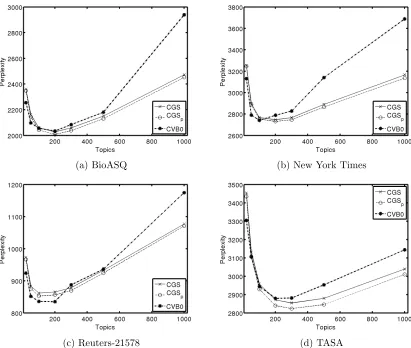
In this experiment we compared the CGS, CGSp and CVB0 algorithms in terms of perplexity,
across different numbers of topics. The motivation here was to examine how the CGSp
method would perform compared to the rest of the algorithms, in a variety of configurations and data sets.
In Appendix E we report also the results of this experiment, comparing the three aforementioned algorithms with Variational Bayes (VB). Since the results for VB were steadily worse, we excluded them from Figure 4, to allow for easier comparison among CVB0, CGS and CGSp. Asuncion et al. (2009) note that the disadvantage of VB versus the other
algorithms can potentially be mitigated via hyperparameter learning.
For this experiment we followed a similar approach to the one described by Asuncion et al. (2009). During training we ran each chain for 200 iterations to obtain a single point estimate of the φandφp distributions. During prediction, using the previously estimatedφ, we ran 200 iterations from one chain for the first half of each document to obtain an estimate of θ. We followed the same approach to compute θp, using φp in that case.6 We then computed perplexity on the second half of each document. Theαk andβv hyperparameters
were fixed across all data sets to uniform values, 0.1 and 0.01 respectively. CVB0 was run with the same parameterization.
Figure 4 shows the perplexity results for all data sets across different settings (20, 50, 100, 200, 300, 500 and 1000 topics) for all methods. Each topics configuration was run for five times, obtaining the average perplexity value. There is a strong interaction between the perplexity scores, the data sets, and the number of topics, probably due to the diverse statistics of the data sets, such as the average document length and the average number of features (i.e., word types) per document (see Table 3 in Section 5.1), that characterize the data sets. All algorithms achieve their lowest perplexity values at around 200 topics.
Despite the peculiarities of individual data sets, we can identify a broad general trend in these results. CVB0 outperforms (marginally in three out of four cases) the other methods in all data sets for lower topic number values: for the BioASQ and TASA data sets this happens up to 50 topics, for the New New York Times data set up to 100 topics, while for Reuters-21578 up to 200 topics. As the number of topics increases though, this behavior is reversed and CGS and CGSp have the upper hand after the aforementioned numbers of
topics.
(a) BioASQ (b) New York Times
(c) Reuters-21578 (d) TASA
Figure 4: Perplexity against number of topics for the CGSp method, standard CGS and
CVB0. Results are taken by averaging over 5 different runs.
A possible explanation for this observation is related to the deterministic nature of CVB0; compared to its stochastic counterpart CGS, CVB0 is more prone to getting stuck in local maxima. As the number of topics increases, we expect the hypothesis space to grow bigger, making it more difficult for CVB0 to find a global optimum. CGS on the other hand, can exploit its stochastic nature to escape local maxima and converge to a better global representation of the data. Therefore, CVB0 seems to be better suited for configurations with a small number of topics (in which case the fact that CVB0 converges a lot faster than CGS as shown by Asuncion et al. (2009) is an additional advantage), while CGS fits better in the opposite case. Similar to the previous section, when comparing CGS and CGSp we