FITTING STATISTICAL DISTRUBTIONS FOR MAXIMUM DAILY RAINFALL AT GKVK STATION

(1)

Available Online at www.ijpret.com 64

INTERNATIONAL JOURNAL OF PURE AND

APPLIED RESEARCH IN ENGINEERING AND

TECHNOLOGY

A PATH FOR HORIZING YOUR INNOVATIVE WORK

FITTING STATISTICAL DISTRUBTIONS FOR MAXIMUM DAILY RAINFALL AT

GKVK STATION

K. N. KRISHNAMURTHY1, R. BHOOMIKA RAJ2, D. M. GOWDA3, M. B. RAJE GOWDA4

1.Associate Professor, University of Agricultural Sciences, GKVK, Bengaluru. 2.Research Scholar, University of Agricultural Sciences, GKVK, Bengaluru. 3.Professor, University of Agricultural Sciences, GKVK, Bengaluru. 4.Professor, University of Agricultural Sciences, GKVK, Bengaluru

Accepted Date: 14/07/2015; Published Date: 01/08/2015

\

Abstract: - Agro-climatic characters play an important role in deciding the cropping pattern of a region. The distribution of rainfall is one such climatic character essential to plan farm activities in a given region. The present study was conducted to know the climatic characterization of GKVK station. The secondary data of weather parameters over a period of 38 years (1976-2013) was collected from AICRP on Agro Meteorology. Among the weather parameters, amount of maximum daily rainfall (mm) was considered to fit appropriate probability distributions. The probability distributions viz., Normal, Log- normal, Gamma (1P, 2P, 3P), Generalized Extreme Value (GEV), Weibull (1P, 2P, 3P), Gumbel and Pareto were used to evaluate the best fit for maximum daily rainfall (mm). Kolmogorov-Smirnov test for the goodness of fit of the probability distributions showed that for majority of the data sets on rainfall at different study periods, Weibull (3P) distribution was found to be the best fit. However, all the data sets were scale dominated which indicated large variation in the distribution of rainfall.

Keywords:Maximum daily rainfall, Probability distributions and Goodness-of-fit test.

Corresponding Author: MR. K. N. KRISHNAMURTHY

Access Online On:

www.ijpret.com

How to Cite This Article:

(2)

INTRODUCTION

Climate is a measure of average pattern of variation in temperature, humidity, atmospheric

pressure, wind speed, precipitation, atmospheric particle count and other meteorological variables in a given region over long periods of time. Climate is different from weather, in that weather only describes the short-term conditions of these variables in a given region. Climate is usually defined as the "average weather" or as the statistical description in terms of the mean and variability of relevant quantities over a period ranging from months to thousands or millions of years. The classical period is 30 years, as defined by the World Meteorological Organization (WMO). These quantities are most often surface variables such as temperature, precipitation, and wind. Climate in a wider sense is the state, including a statistical description, of the climate system. Rainfall is one of the most important natural input resources to crop production. Its occurrence and distribution is erratic. Analysis of rainfall data strongly depends on its distribution pattern. It has long been a topic of interest in the fields of Agricultural Statistics in establishing a probability distribution that provides a good fit to daily rainfall data. Several studies have been conducted in India and abroad on rainfall analysis and best fit probability distribution functions such as normal, lognormal, Weibull and gamma type distributions were identified.

The annual and seasonal analysis of rainfall will give general idea about the rainfall pattern of the region, whereas the monthly as well as weekly analysis of rainfall will be of much use as far as agricultural planning is concerned.Knowledge of the distribution of rainfall is essential for successful farming.

Gregory et al. (2007) demonstrated the feasibility of ﬁtting cell-by-cell probability distributions

to grids of monthly interpolated, Continent-wise data and showed that the gamma distribution was well suited. Suhaila and Jemain (2007) showed that Mixed Exponential was found to be the most appropriate distribution for describing the daily amount of rainfall in Peninsular Malaysia. Lars and Vogel (2008) studied the distribution of wet-day daily rainfall and identified that the 2-parameter Gamma (2P) distribution as the most likely candidate distribution based on

traditional goodness of fit tests. Deka et al. (2009) compared the goodness of fit test results

and generalized logistic distribution was empirically proved to be the most appropriate distribution for describing the annual maximum rainfall series for the majority of the stations in North East India. Sharma and Singh (2010) analyzed the maximum daily rainfall data of Pantnagar for a period of 37 years for annually, seasonally, monthly and weekly, and the best

fitted probability distribution was identified using goodness of fit tests. Manikandan et al.

(3)

Available Online at www.ijpret.com 66 Campus. Chi-square values revealed that the log-normal distribution was the best fit probability

distribution for annual one day maximum rainfall. Bhim Singh et al. (2012) analyzed the daily

rainfall data of 39 years (1973-2011) in Jhalarapatan area of Rajasthan and log-Pearson type-III distribution was found to be the best fit probability distribution. Oseni and Femi (2012) have fitted several types of statistical distributions to describe rainfall distribution in Ibadan metropolis over a period of 30 years. Mayooran and Laheetharan (2014) have identified best fit probability distributions among 45 standard probability distributions to model annual maximum rainfall in Colombo district for a period of 110 years.The present study was planned for establishing the methodology for identifying the best fit probability distribution formaximum daily rainfall.

MATERIAL AND METHODS

The present study was conducted to know the pattern of rainfall distribution at Gandhi KrishiVignana Kendra (GKVK) station. The station, GKVK is located at Bengaluru Urban District of Bengaluru North Taluk. It belongs to the Eastern Dry zone (Zone-V). The geographical

co-ordinates of this station are 77o35’ longitude, 12o58’ latitude and 930 amsl altitude. The Eastern

dry zone includes Kolar, Tumakuru, Bengaluru (Urban), Bengaluru (Rural), Chikkaballapur and Ramanagara. The zone has an average annual rainfall of 944mm (1976-2013). Major crops grown in this zone are ragi, groundnut, rice and maize.

The present study was based on the secondary data on rainfall over a period of 38 years (1976-2013) which was collected from AICRP on Agro Meteorology, University of Agricultural Sciences, GKVK, Bengaluru.

Fitting probability distributions

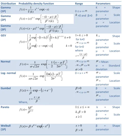
The standard probability distributions viz. normal, log-normal, gamma (1P, 2P and 3P), Weibull (1P, 2P and 3P), Gumbel, Paretoand generalised extreme value (GEV) were identified to evaluate the best fit probability distribution for maximum daily rainfall. The description of various probability density functions, range of the variable and the parameters involved are presented in Table 1.

Description of parameters:

 Shape parameter

(4)

Table 1: Description of various probability density functions with range of variable and parameters.

Distribution Probability density function Range Parameters Gamma

(1P) ( ) exp( )

1 )

( x 1 x

k x

f k 



 

0 ≤ x <+

k_{>0 and β>0}

K = Shape parameter

β = Scale parameter

µ = Location parameter

Gamma

(2P) _

       ) ( / ) ( exp ) ( ) ( 1 k k x x

f k _k

 

 

Gamma

(3P) _

          ) ( / ) ( exp ) ( ) ( 1 k k x x f k k    

GEV

_

_{ }

_





               _ _     0 ) exp( exp 1 0 1 1 exp 1 ) ( / 1 1 1 k z z k kz kz x f k k   0 1k z for k≠0 -< x <+ for k=0 where  ) (   x z

k₌ _Shape

parameter

µ = Location parameter

Normal





     _ 

 ₂ 2

2 2 1 exp 2 1 ) (     x x f

-_{< x <+} -<<+

0





_{= Mean}

σ = Standard deviation

Log- normal



 



      

 ₂ 2

2 ln exp 2 1 ) (     x x x

f 0 < x < +

 ₌ _Scale parameter

₌ _Location

parameter

Gumbel



z



e z x

f( ) 1 exp  



Where,     x z 0  

-< x <+

₌ _Location

parameter

Pareto

1 ) (  _k_

k k x f   1 0 , 1       x k x 

k = Shape parameter

Weibull

(1P)

 

 



x x

x

f( ) 1exp

0 0   

x β = Shape

(5)

 Scale parameter

The scale parameter of a distribution determines the scale of the distribution function. The larger the scale parameter, the more spread out the distribution. The examples of scale parameters include variance and standard deviation.

 Location parameter

The location parameter determines the position of central tendency of the distribution along the x-axis.. The location parameter defines the shift of the data. Examples of location parameters include the mean, median, and the mode.

Kolmogorov- Smirnov test (K-S test) for testing the goodness of fit

The goodness of fit test measures the discrepancy between observed values and the expected values. Kolmogorov- Smirnov test was used to test for the goodness of fit.

In the present investigation, the goodness of fit test was conducted at = 0.05 level of

significance. It was applied for testing the following hypothesis:

H0: The maximum daily rainfall data follows a specified distribution.

H1: The maximum daily rainfall data does not follow a specified distribution.

This test is used to decide whether a sample comes from a hypothesized continuous probability density function. It is based on the empirical distribution function i.e., on the largest vertical difference between the theoretical and empirical cumulative distribution function.

 

      _  _  

i n i _n F Xi

i n i X F

D max 1,

1 Weibull (2P) k k x x k x f _                  exp ) ( 1

0 ≤ x <+

0 , ,  k

k = Shape parameter

₌ _Scale

parameter

₌ _Location

parameter

(6)

Where, Xi = Random sample, i= 1, 2,…, n.

 

n X F

CDF n

1  

[Number of observations ≤ x]

Identification of best fit probability distribution.

The KS test was used to identify the best fit probability distribution for maximum daily rainfall for different data sets. The test statistic of the test was computed and tested at (α = 0.05) level of significance. Among all the fitted probability distributions for maximum daily rainfall, the distribution with lowest test statistic value and highest p-value was considered as the best fit.

RESULTS AND DISCUSSION

The methodology presented above was applied to the 38 years weather data in which maximum rainfall in millimetres were collected from AICRP on agro meteorology located at UAS, GKVK, Bengaluru. Accordingly, the data was classified into 28 data sets as mentioned in Table-2. These 28 data sets were classified as 1 annual, 1 seasonal, 5 seasonal months and 21standard meteolorogical weeks to study the distribution pattern at different levels.

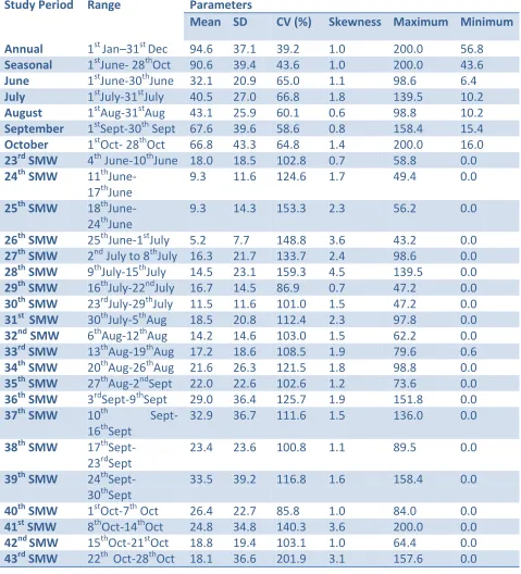
Descriptive statistics of maximum daily rainfall

The summary of statistics such as highest, lowest, mean, standard deviation, skewness and coefficient of variation values of maximum daily rainfall are presented in Table 2. The results show that both annual and seasonal maximum daily rainfall was observed to be 200 mm. Monthly maximum daily rainfall during monsoon season ranged from 98.6 mm to 200 mm while weekly maximum daily rainfall was between 43.2 mm to 200 mm. It was also observed that the minimum daily rainfall was 56.8 mm annually, 43.6 mm seasonally and it ranged from 6.4 mm to 16 mm monthly. For all the weeks, the minimum rainfall was found to be 0.0 mm.

Annual mean of the maximum daily rainfall was found to be 94.6 mm, whereas for overall south-west monsoon seasonal months, it was 90.6 mm. During the seasonal months, the mean of the maximum daily rainfall ranged from 32.1mm to 67.6 mm while for weekly, it varied from 5.2 mm to 33.5 mm.

(7)

Table 2: Summary statistics for maximum daily rainfall (mm)

Study Period Range Parameters

Mean SD CV (%) Skewness Maximum Minimum

Annual 1st Jan–31st Dec 94.6 37.1 39.2 1.0 200.0 56.8

Seasonal 1stJune- 28thOct 90.6 39.4 43.6 1.0 200.0 43.6

June 1stJune-30thJune 32.1 20.9 65.0 1.1 98.6 6.4

July 1stJuly-31stJuly 40.5 27.0 66.8 1.8 139.5 10.2

August 1stAug-31stAug 43.1 25.9 60.1 0.6 98.8 10.2

September 1stSept-30th Sept 67.6 39.6 58.6 0.8 158.4 15.4

October 1stOct- 28thOct 66.8 43.3 64.8 1.4 200.0 16.0

23rd SMW 4th June-10thJune 18.0 18.5 102.8 0.7 58.8 0.0

24th SMW 11th June-17thJune

9.3 11.6 124.6 1.7 49.4 0.0

25th SMW 18th June-24thJune

9.3 14.3 153.3 2.3 56.2 0.0

26th SMW 25thJune-1stJuly 5.2 7.7 148.8 3.6 43.2 0.0

27th SMW 2nd July to 8thJuly 16.3 21.7 133.7 2.4 98.6 0.0

28th SMW 9thJuly-15thJuly 14.5 23.1 159.3 4.5 139.5 0.0

29th SMW 16thJuly-22ndJuly 16.7 14.5 86.9 0.7 47.2 0.0

30th SMW 23rdJuly-29thJuly 11.5 11.6 101.0 1.5 47.2 0.0

31st SMW 30thJuly-5thAug 18.5 20.8 112.4 2.3 97.8 0.0

32nd SMW 6thAug-12thAug 14.2 14.6 103.0 1.5 62.2 0.0

33rd SMW 13thAug-19thAug 17.2 18.6 108.5 1.9 79.6 0.6

34th SMW 20thAug-26thAug 21.6 26.3 121.5 1.8 98.8 0.0

35th SMW 27thAug-2ndSept 22.0 22.6 102.6 1.2 73.6 0.0

36th SMW 3rdSept-9thSept 29.0 36.4 125.7 1.9 151.8 0.0

37th SMW 10th Sept-16thSept

32.9 36.7 111.6 1.5 136.0 0.0

38th SMW 17th Sept-23rdSept

23.4 23.6 100.8 1.1 89.5 0.0

39th SMW 24th Sept-30thSept

33.5 39.2 116.8 1.6 158.4 0.0

40th SMW 1stOct-7th Oct 26.4 22.7 85.8 1.0 84.0 0.0

41st SMW 8thOct-14thOct 24.8 34.8 140.3 3.6 200.0 0.0

42nd SMW 15thOct-21stOct 18.8 19.4 103.1 1.0 64.4 0.0

(8)

Available Online at www.ijpret.com 71 Meteorological Weeks (SMW’s), the rainfall variation was found to be very high ranging from 86.9 to 201.9 per cent.

The coefficient of skewness for all the data sets ranged from 0.6 to 4.5 indicating positive skewness. From this result, we can conclude that in all the data sets the average rainfall for the period exceeded the modal value.

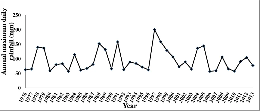
Figure 1 shows the year wise variation in annual maximum daily rainfall from 1976-2013. It ranged from 56.8 mm (in 2006) to 200 mm (in 1997). The minimum of the maximum daily

rainfall, i.e., 56.8 mm occurred during 10th SMW (5th Mar-11th Mar) and the maximum of the

maximum daily rainfall of 200 mm occurred during the 41st SMW (8th Oct-14th Oct).

Fig 1: Variation in Maximum daily rainfall (mm) over a study period

Fitting the probability distributions

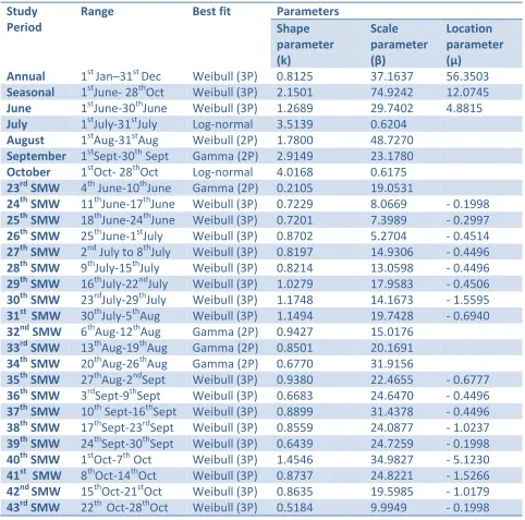
Study period probability distribution using goodness of fit tests is given in the Table 3. It was observed from the table that Weibull (3P) distribution was the best fit probability distribution for majority of the Standard Meteorological Weeks, for the annual, seasonal and June month study periods. Log-normal distribution fitted well for July and October months while, Weibull (2P) was the best fit for August month. Gamma (2P) was observed to be the best fit for seasonal

month of September along with the standard weeks such as 23rd, 32nd, 33rd and 34th. Weibull

(3P) distribution fitted well for majority of the data sets since the distribution provides a flexible representation of a variety of shapes. Majority of the study periods were scale-dominated which indicated large variation in the distribution of rainfall.

0 50 100 150 200 250

A

nn

ual

m

ax

im

um

dail

y

rai

nf

al

l

(m

m

)

(9)

Available Online at www.ijpret.com 72 The distribution parameters helped to determine the pattern of the rainfall distribution in the study region. The joint interpretation of shape and scale parameters conveys the distribution of values in the modeled rainfall data at each location allowing the interpreter a qualitative assessment of the amount and stability of rainfall throughout the season. These parameters reflect the modeled rainfall, and as such also contain errors inherent in the modeled history.

Table 3: Study period wise probability distribution using goodness of fit tests.

Study Period

Range Best fit Parameters Shape parameter (k)

Scale parameter (β)

Location parameter (µ)

Annual 1st Jan–31st Dec Weibull (3P) 0.8125 37.1637 56.3503

Seasonal 1stJune- 28thOct Weibull (3P) 2.1501 74.9242 12.0745

June 1stJune-30thJune Weibull (3P) 1.2689 29.7402 4.8815

July 1stJuly-31stJuly Log-normal 3.5139 0.6204

August 1stAug-31stAug Weibull (2P) 1.7800 48.7270

September 1stSept-30th Sept Gamma (2P) 2.9149 23.1780

October 1stOct- 28thOct Log-normal 4.0168 0.6175

23rd SMW 4th June-10thJune Gamma (2P) 0.2105 19.0531

24th SMW 11thJune-17thJune Weibull (3P) 0.7229 8.0669 - 0.1998

25th SMW 18thJune-24thJune Weibull (3P) 0.7201 7.3989 - 0.2997

26th SMW 25thJune-1stJuly Weibull (3P) 0.8702 5.2704 - 0.4514

27th SMW 2nd July to 8thJuly Weibull (3P) 0.8197 14.9306 - 0.4496

28th SMW 9thJuly-15thJuly Weibull (3P) 0.8214 13.0598 - 0.4496

29th SMW 16thJuly-22ndJuly Weibull (3P) 1.0279 17.9583 - 0.4506

30th SMW 23rdJuly-29thJuly Weibull (3P) 1.1748 14.1673 - 1.5595

31st SMW 30thJuly-5thAug Weibull (3P) 1.1494 19.7428 - 0.6940

32nd SMW 6thAug-12thAug Gamma (2P) 0.9427 15.0176

33rd SMW 13thAug-19thAug Gamma (2P) 0.8501 20.1691

34th SMW 20thAug-26thAug Gamma (2P) 0.6770 31.9156

35th SMW 27thAug-2ndSept Weibull (3P) 0.9380 22.4655 - 0.6777

36th SMW 3rdSept-9thSept Weibull (3P) 0.6683 24.6470 - 0.4496

37th SMW 10th Sept-16thSept Weibull (3P) 0.8899 31.4378 - 0.4496

38th SMW 17thSept-23rdSept Weibull (3P) 0.8559 24.0877 - 1.0237

39th SMW 24thSept-30thSept Weibull (3P) 0.6439 24.7259 - 0.1998

40th SMW 1stOct-7th Oct Weibull (3P) 1.4546 34.9827 - 5.1230

41st SMW 8thOct-14thOct Weibull (3P) 0.8737 24.8221 - 1.5266

42nd SMW 15thOct-21stOct Weibull (3P) 0.8635 19.5985 - 1.0179

(10)

CONCLUSION

The present study revealed the distribution pattern of Maximum daily rainfall at GKVK station using appropriate best fit probability distributions. Kolmogorov-Smirnov test statistic and p-values of the probability distributions showed that for majority of the data sets of rainfall at different study periods, Weibull (3P) distribution was found to be the best fit among the 11 fitted distributions. However, majority of the data sets were scale dominated which indicated large variation in the distribution of rainfall.

REFERENCES

1. Bhim Singh, Deepak Rajpurohit, Amol Vasishth and Jitendra Singh., 2012, Probability Analysis

For Estimation Of Annual One Day Maximum Rainfall of Jhalarapatan Area Of Rajasthan, India. Plant Archives, 12(2): 1093-1100.

2. Deka S and Borah, M., 2009, Distribution of Annual Maximum Rainfall Series of North-East

India, European Water Publications, 27/28: 3–14.

3. Gregory, J. Husak., Joel Michaelsen and Chris Funk., 2007, Use Of The Gamma Distribution To

Represent Monthly Rainfall In Africa For Drought Monitoring Applications. International Journal of Climatology, 27: 935–944.

4. Lars S. Hanson and Vogel Richard, 2008, the Probability Distribution of Daily Rainfall in The

United States. Proceedings of World Environmental and Water Resources Congress, 1-10.

5. Manikandan, M., Thiyagarajan, G. And Vijaya Kumar, G., 2011, Probability Analysis For

Estimating Annual One Day Maximum Rainfall In Tamil Nadu Agricultural University, Madras Agricultural Journal, 98(1/3): 69-73.

6. Mayooran, T and Laheetharan, A., 2014, the Statistical Distribution of Annual Maximum

Rainfall In Colombo District, Sri Lankan Journal Of Applied Statistics, 15-2:107-130.

7. Oseni, B. Azeez and Femi J. Ayoola., 2012, Fitting The Statistical Distribution For Daily Rainfall

In Ibadan, Based On Chi-Square And Kolmogorov-Smirnov Goodness-Of-Fit Tests, European Journal Of Business And Management, 4(17): 62-70.

8. Sharma, M.A., and Singh, J.B., 2010, Use of Probability Distribution in Rainfall Analysis, New

(11)

9. Suhaila And Jemain Abdul Aziz., 2007, Fitting The Statistical Distributions To The Daily