SIMULATION OF REDUCING SENSOR COVERAGE AREA OF WIRELESS LAN USING TIME OFF SCHEME

(1)

Available Online at www.ijpret.com 1487

INTERNATIONAL JOURNAL OF PURE AND

APPLIED RESEARCH IN ENGINEERING AND

TECHNOLOGY

A PATH FOR HORIZING YOUR INNOVATIVE WORK

SIMULATION OF REDUCING SENSOR COVERAGE AREA OF WIRELESS LAN

USING TIME OFF SCHEME

MILIND K TATTE

Nagar Parishad Polytechnic, Achalpur.

Accepted Date: 15/03/2016; Published Date: 01/05/2016

\

0

Abstract: There are several localized sensor area coverage protocols for heterogeneous sensor, each with arbitrary sensing and transmission radii. The approach has a very small communication overhead since prior knowledge about neighbour existence. Each node select a random time out and listen to message send by other nodes before the time out expire. Sensor node whose sensor area is not fully covered, when the deadline expire decide to remain active for the considered round and transmit an activity message announcing it. Covered nodes decide to sleep, with or without transmitting a withdrawal message to inform neighbours about the status. After hearing from more neighbours, active sensors may observe that they became covered and may decide to alter their original decision and transmit a retreat message. Our simulations show a largely reduced message overhead while preserving coverage quality for the ideal MAC/physical layer.

Keywords: Sensor networks, Area coverage, Network connectivity, localized algorithm, ART, TGJD

Corresponding Author: MR. MILIND K TATTE Access Online On:

www.ijpret.com

How to Cite This Article:

(2)

Available Online at www.ijpret.com 1488 INTRODUCTION

The problem considered is about sensors making decisions whether or not to turn off so that the whole area remains fully covered and the subset of active nodes remains connected. Therefore, the sensor area coverage problem is to determine a small number of active and connected sensors that still cover the same area as the fully deployed set. In centralized solutions, the information about topological changes in dynamic networks must be propagated throughout the network to maintain the information needed for each node to make a decision. In distributed solutions, protocols relax this information propagation and use memorization at nodes. It also used unbounded delays. In a Localized solutions have significantly lower communication overhead since no global view of the network is required. In a localized protocol, each node makes its activity status decision solely based on the decisions made by its communication neighbours. Moreover, in a fully localized protocol, decisions are not impacted by distant nodes Our solutions rely on an extremely reduced communication overhead[07] in order to be suitable also for highly dense networks. No neighbour discovery is needed. Nodes wait for random time-out duration while receiving decision messages from neighbours. The sensor evaluates its coverage and connectivity by active neighbours and decides whether or not to be active when the time out expires. Active sensors inform neighbours, whereas decisions to sleep may or may not be announced. After making a decision to be active, nodes may hear from more active neighbours, and their sensing area may then become fully covered. Such nodes may then change their minds by sending a retreat message to their neighbours.

1.1 Problem Definition

(3)

to optimize energy usage during query execution would be for the network to self-organize, in response to a query, into a logical topology involving a minimum number of sensor nodes that is sufficient to process the query. Only the sensors in the logical topology would participate (communicate with each other) during the query execution. This is a very effective strategy for energy conservation, especially when there are many more sensors in the network than are necessary to process a given query.

1.2 System Design

(4)

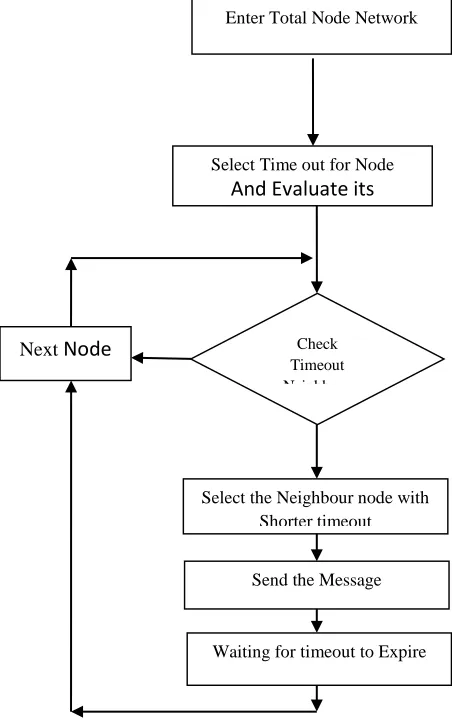
Available Online at www.ijpret.com 1490 Fig 01:-.Flow-Diagram of the system

1.3 Detailed Design Structure

We describe here three specific ways denoted as,

Random Time out (RT)

Extendable Random Time out (ERT)

Activity-Aware Time out (AAT)

The simplest way for deciding the time-out duration is to select a random number in a fixed interval [0, TOW],[ ] where TOW is the integer number of slots denoting the maximum possible duration for any node (assumed to be fixed and the same for all nodes). This method will be

Enter Total Node Network

Select Time out for Node And Evaluate its

Coverage

Check Timeout Neighbour

Select the Neighbour node with Shorter timeout

Send the Message

(5)

referred to as the RT method. It is anticipated that the need to be active will decrease after receiving activity decisions from sensing neighbours. Such messages can be incorporated into a time-out function to modify it “on the fly” in various ways. One way is to observe the amount of sensing area overlap [08]. Since exact calculation is time consuming for an actual implementation, we considered a simplified version where the node chooses a number of random points inside its own sensing area. It then evaluates if any of its already known neighbours is able to sense it. Nodes initially select random time outs in [0, M]. After each received activity message from its sensing neighbours, a node calculates the ratio R (thus, R is in [0, 1]) of the random points that becomes covered by them. The time-out duration is then modified to M +R (TOW-M). Thus, the time out is extended after each received message. This

method is referred to as method ERT. We used M= 2

TOW

in our experiments, which appeared best after trying several options. Our third method AAT is motivated by the expected energy balance of previously active nodes when the new round starts. In the first round, nodes select random time outs in [0, TOW], as in method RT. Nodes active in the previous round should attempt to avoid repeating this by selecting longer time-out durations. A node u that has been

active during a > 0 consecutive rounds will pick up its time out within the last 1 a1 portion of the time-out window. The node selects Random within [0, 1] and then, as time duration, selects the rounded value of timeoutu= TOW - Random x TOW/ a + 1

In a symmetric manner, the longer nodes are passive, the shorter their time outs should be in order to incite them to get active. Then, a node u that has been passive during p consecutive

rounds will pick up its time out within the first 1 1



p _{portion of the time-out window. In this case,}

u will compute its time out as follows:

timeoutu= Random x TOW/ p + 1

We used several approaches for the activity counter evolution. Basically, when a node changes its status, it can reset every counter or not. We opted for a variant with an overall counter, which is incremented when the node is active and decremented when the node decides to be passive. Therefore, in our implementation, we actually had one variable, whose absolute value was used as a value for “a” or “p”, according to its sign.

(6)

@ Activity only (AO). Only nodes that decide to be active send a (exactly one) message.

@ Activity and withdrawal (AW). Every node sends exactly one message, which corresponds to its decision, an activity acknowledgment for an active status or a withdrawal before entering a sleep mode.

@ Activity and retreat (AR). Nodes that decide to be active send their decisions, whereas nodes that decide to sleep do not. Active nodes, however, can later on learn that they are covered with the help of newly announced active nodes and may decide to “change their minds” and to enter the sleep mode; such nodes send also one retreat message.

@ Activity, withdrawal, and retreat, (AWR). All decisions by all nodes are transmitted; thus, each node sends one message corresponding to the original decision on the active or sleep status. Nodes with an originally active decision may reconsider it later on and switch to the sleep mode and possibly send one retreat message..

2.0 IMPLEMENTATION

(7)

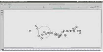
provide initial position of node. Set a TCP/IP connection between the all 25 nodes when one node change the position, it colour will change while moving. Observe all node position with respective original location of node. Followings are some screenshots which are simulated in nam animator gives visualation effect of tcl file.

Fig 02:- Display of Nodes placement in NS-2

The fig.02 provides display and position of nodes. The nodes are placed with respect to values provided in tcl file.

Fig. 03:- Nodes broadcasting data-packets

(8)

Available Online at www.ijpret.com 1494 Fig.04:-Nodes displacement from their positions

The fig.04 provides explanation of nodes displacement from their positions. The nodes are moving within the region as well as transferring data.

Fig.05:- Node is shown as deleted

In the fig. 05, node is displayed as deleted node although displaying in the plane. The yellow color displays its deletion from the region.

Fig.06:- Node changing the region while making movement.

(9)

Available Online at www.ijpret.com 1495 Fig.07:- : Packet transfer within nodes

The figure shows the packet transfer from various nodes. In this figure, p-it displays the transfer from node12 to node 0.

Fig.08:- Summary of display regarding nodes.

The fig.08 shows the packet transfer, deleted node and node changing region.

2.1 Result

(10)

Available Online at www.ijpret.com 1496 No of No d es Tot al Se n d in g(p) Tot al R eceive d (p) R ou te p ackets _PDF (In %) NRL De la y

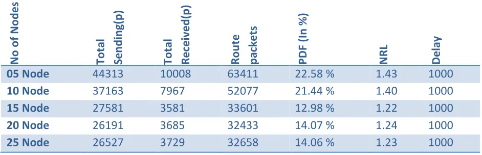
05 Node 44313 10008 63411 22.58 % 1.43 1000 10 Node 37163 7967 52077 21.44 % 1.40 1000 15 Node 27581 3581 33601 12.98 % 1.22 1000 20 Node 26191 3685 32433 14.07 % 1.24 1000 25 Node 26527 3729 32658 14.06 % 1.23 1000

Table 1: Comparative Analysis for different number of nodes

The Terminology related with table is as under:

Packet delivery Fraction: The ratio of the number of delivered data packet to the destination. This illustrates the level of delivered data to the destination.



(Number of packet received) /



(Number of packet send

The greater value of packet delivery ratio means the better performance of the protocol.

End-to-end Delay: The average time taken by a data packet to arrive in the destination. It also includes the delay caused by route discovery process and the queue in data packet transmission. Only the data packets that successfully delivered to destinations that counted.



(Arrive time – send time) /



(Number of connections)

The lower value of end to end delay means the better performance of the protocol.

Packet Lost: The total number of packets dropped during the simulation.

Packet lost = Number of packet send – Number of packet received. The lower value of the packet lost means the better performance of the protocol.

(11)

Available Online at www.ijpret.com 1497 Fig 09:- Analysis Graph between Total Send, Receive and Route packet

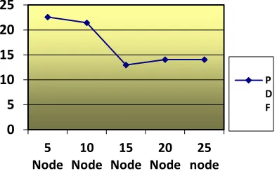
Fig 10:- Analysis Graph between No of Nodes and PDF

Fig. 11:- Analysis Graph between No of Nodes and NRL

0 20000 40000 60000 80000 100000 120000 140000 5 Node 10 Node 15 Node 20 Node 25 Node Route Packet Total Received Total Send 0 5 10 15 20 25 5 Node 10 Node 15 Node 20 Node 25 node

Number of Nodes

P D F 0 5 10 15 20 25 5 Node 10 Node 15 Node 20 Node 25 node

Number of Nodes

(12)

Available Online at www.ijpret.com 1498 3.0 CONCLUSION

We have proposed a localized algorithm for maintaining connected area coverage under various ratios of communicating and sensing radii. In addition to providing different number of node in sensor Network. When there was a large nodes are present in network, the route packet delivery from source to destination is high, but it was reduces even though the number of node is may increased in network. When we apply the scheme of time delay for each node, we observed NRL factor of network is reduces. It means low collision in network. Here we plan to extend the work by given exact placing location of node in large network so it work as a active agent and normalised the communication overheads.

REFERENCES

1. Elson, J., Romer, K.: Wireless sensor networks: A new regime for time synchronization. In: The First Workshop on Hot Topics In Networks (HotNets-I). (2002)

2. Xue, F., Kumar, P.R.: The number of neighbors needed for connectivity of wireless networks. Wireless Networks (2003)

3. Cox, D.: Renewal Theory. Methuen and Co. LTD Science Paperbacks (1970)

4. Elsayed, K.M.F., Perros, H.G.: The superposition of discrete-time markov renewal processes with an application to statistical multiplexing of bursty traffic sources. Applied Mathematics and Computation (Kluwer Academic Publisher) (2000)

5. J. Carle, A. Gallais, and D. Simplot-Ryl, “Preserving Area Coverage in Wireless Sensor Networks by Using Surface Coverage Relay Dominating Sets,” Proc. 10th IEEE Symp. Computers and Comm. (ISCC), 2005.

6. A. Gallais, J. Carle, D. Simplot-Ryl, and I. Stojmenovic, “Localized Sensor Area Coverage with Low Communication Overhead,” Proc. Fourth IEEE Int’l Conf. Pervasive Computing and Comm. (PerCom), 2006.

7. C.-F. Hsin and M. Liu, “Network Coverage Using Low Duty- Cycled Sensors: Random & Coordinated Sleep Algorithms,” Proc. Third Int’l Symp. Information Processing in Sensor Networks (IPSN), 2004.

8. J. Jiang and W. Dou, “A Coverage Preserving Density Control Algorithm for Wireless Sensor Networks,” Proc. Third Int’l Conf. Ad-Hoc Networks and Wireless (ADHOC-NOW), 2004.

(13)

10. D. Tian and N. Georganas, “A Coverage-Preserving Node Scheduling Scheme for Large Wireless Sensor Networks,” Proc. First ACM Int’l Conf. Wireless Sensor Networks and Applications (WSNA ’02), pp. 32-41, 2002.

11. G. Xing, X. Wang, Y. Zhang, C. Lu, R. Pless, and C. Gill, “Integrated Coverage and Connectivity Configuration for Energy Conservation in Sensor Networks,” ACM Trans. Sensor Networks, vol. 1, no. 1, pp. 36-72, 2005.

12. T. Yan, T. He, and J.A. Stankovic, “Differentiated Surveillance Service for Sensor Networks,” Proc. ACM Conf. Embedded Networked Sensor Systems (SenSys), 2003.

13. F. Ye, G. Zhong, J. Cheng, S. Lu, and L. Zhang, “PEAS: A Robust Energy Conserving Protocol for Long-Lived Sensor Networks,” Proc. 23rd Int’l Conf. Distributed Computing Systems (ICDCS), 2003.

14. H. Zhang and J.C. Hou, “Maintaining Sensing Coverage and Connectivity in Large Sensor Networks,” Ad Hoc & Sensor Wireless Networks, vol. 1, pp. 89-123, 2005.

15. S. Meguerdichian, F. Koushanfar, G. Qu, and M. Potkonjak. Exposure in wireless ad-hoc sensor networks. In Proceedings of the International Conference on Mobile Computing and Networking (MobiCom), 2001.199

16. S. Shakkottai, R. Srikant, and N. Shroff. Unreliable sensor grids: Coverage, connectivity and diameter. In Proceedings of INFOCOM (to appear), 2003.

17. S. Slijepcevic and M. Potkonjak. Power efficient organization of wireless sensor networks. In Proc. Of IEEE Intl. Conf. on Communications (ICC), 2001.

18. X. Wang, G. Xing, Y. Zhang, C. Lu, R. Pless, and C. Gill, “Integrated coverage and connectivity configuration in wireless sensor networks,” in Proceedings of ACM Conference on Embedded Networked Sensor Systems (SenSys), Los Angeles, CA, USA, 2003, pp. 28–39.

19. F. Ye, G. Zhong, S. Lu, L. Zhang, Energy Efficient Robust Sensing Coverage in Large Sensor Networks, Technical Report.

20. C.Intagagonwiwat, R.Govindan, and D.Estrin, Directed Diffusion: A Salable and Robust Communication Paradigm for Sensor Networks, Proc. of the AMC Mobicom’00, Boston, MA, 2000.