An Efficient Approach for Bottleneck Resource(s) Detection Problem in the Multi-objective Dynamic Job Shop Environments

(1)

Please cite this article as: N. Nahavandi, M. Abbasian,An Efficient Approach for Bottleneck Resource(s) Detection Problem in the Multi-objective Dynamic Job Shop Environments, International Journal of Engineering (IJE), TRANSACTIONS C: Aspetcs Vol. 29, No. 12, (December 2016) 1691-1703

International Journal of Engineering

J o u r n a l H o m e p a g e : w w w . i j e . i r

An Efficient Approach for Bottleneck Resource(s) Detection Problem in the

Multi-objective Dynamic Job Shop Environments

N. Nahavandi*_{, M. Abbasian}

Faculty of Industrial and Systems Engineering, Tarbiat Modares University, Tehran, Iran

P A P E R I N F O

Paper history:

Received 18 March 2016

Received in revised form 06 June 2016 Accepted 02 June 2016

Keywords: Energy Saving

Multi-objective Dynamic Job Shop Theory of Constraints

Bottleneck Resource Bottleneck Resource Detection

A B S T R A C T

Nowadays energy saving is one of the crucial aspects in decisions. One of the approaches in this case is efficient use of resources in the industrial systems. Studies in real manufacturing systems indicating that one or more machines may also act as the Bottleneck Resource/ Resources (BR). On the other hand, according to the Theory of Constraints (TOC), the efficient use of resources in manufacturing systems is limited by the capacity of the BR(s). Hence, in order to improve the performance of such systems, the BR(s) should be identified and assessed and improved using capacity of such resources to the greatest extent possible. Studies indicating that Bottleneck Resource Detection (BRD) problem in the ―Multi-Objective and the Dynamic conditions‖ of job-shop is an important issue which has not been studied so far due to its computational complexity. Hence, the development of an efficient approach to identify and assess BRs in Multi-objective Dynamic Job Shop (MODJS) has been considered as the subject of this paper. In this article, a BRD method based on the Taguchi method for MODJS (TM-MODJS) has been developed. This method takes the objectives of the MODJS as estimated indices and carries out typical and finite number of experiments by combining different suitable dispatching rules to detect BR(s) which have the greatest effect on the estimated index. Comparing the results indicates effectiveness of the developed method especially in scheduling which results in a reasonable time.

doi: 10.5829/idosi.ije.2016.29.12c.08

NOMENCLATURE

Index Operation,

Each job (e.g. the job ) enters the shop for process a nonzero time.

Job If the job is performed on the machine prior to the job , = 1; otherwise, = 0.

Operation

machine Variables

Parameters the job‘s completion time on the machine

great and positive number the operation process time from the job is on the machine

Number of jobs, the scheduling scheme for machine

Number of machines, objective value

1. INTRODUCTION1

Real manufacturing systems generally have Bottleneck Resource (BR) [1]. According to concepts of TOC, the throughput of the manufacturing systems is limited by the capacity of the BR(s) [2]. In a Multi-Objective

1_{*Corresponding Author‘s Email: [email protected] (N.}

Nahavandi)

Dynamic Job Shop (MODJS) environment

( | | ∑ ̅ ̅ ), one or a

(2)

2. LITERATURE REVIEW

2. 1. Definition and Types of BR(S) BR(s) is machine(s) which prevent better function of the system. In a classification by Hinckeldeyn et al. [3], different types of BR(s) are: capacity, parts, flexibility, layout, budget, information, and know-how. On the other view, BR(s) is classified in three categories (Figure 1). In Simple BR only one of the machines acts as a bottleneck. In Multiple BRs, more than one machine acts as a bottleneck. But these bottlenecks are fixed throughout the considered period of time. In the Shifting BR, there is not just one bottleneck for the entire period, but during the period the bottleneck shifts from one machine to another [4].

2. 2. Literature Review BRD Methods Roser et al. [5] have identified and classified all the BRD methods up to 2002, in the following methods:

 UF (Utilization Factor),

 QSFM (Queue Size in Front of Machine),

 WTFM (Waiting Time in Front of Machine) and

 AP (Active Period).

In another research, Roser et al. [5] have detected BR by calculating active periods of machines and called it Shifting Bottleneck Detection (SBD).

(a) Simple BR

(b) Multiple BRs

(c) Shifting BRs

Figure 1. Simple, Multiple and Shifting BRs [4]

(3)

shop manufacturing systems which have capacity. Their dynamic conception includes demand changes and estimated production times. Glock and Jaber [21] studied the effects of learning and forgetting graphs parameters in a two-level serial manufacturing systems. They also investigated the phenomenon of shifting BR(s). They showed taking advantage of learning may lead to BR(s). By predicting the position of system‘s potential BR, this enables the system to take flexible reaction in shifting BR(s).

Hinckeldeyn et al. [3] strived to develop BR management from manufacturing discussions to engineering process and product design discussions by presenting a new conception of BR management. They presented this new conception using system theory simulation approach. Abbasian et al. [22] investigated FJS considering resource availability constraints. They presented an intelligent GA to solve it. In order to limit BR(s), they used parallel machine implementation approach, but they did not propose a method for BRD problem and postponed it to their future studies. Literature review indicates that BRD problem even in

CJS is still in the center of attention for researchers as one of the recurrent research areas [3, 11]. Also, the BRD problem in the ―Multi-Objective and the Dynamic‖ conditions of job-shop is an important issue which has not been studied in the previous literature due to its computational complexity.

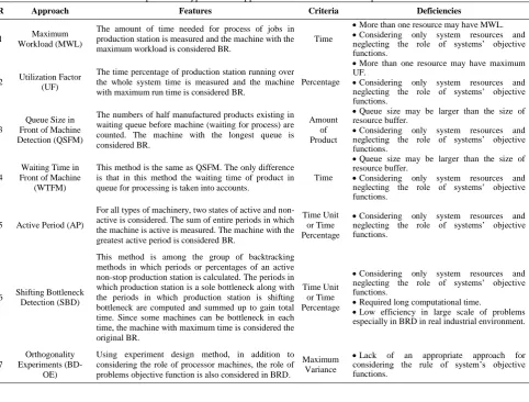
2. 3. BRD Methods Classifications In order to rigorous comparisons among the different approaches reported in the literature, typical BRD methods available in the literature for CJS problem are classified and analyzed in Table 1. In general, regarding Table1, it can be deduced that there are three common approaches for BRD in CJS, as follows:

 First group of BRD approaches (like MWL and UF) detect BR by measuring efficiency or workload. A machine with the greatest efficiency or workload is introduced as the BR. These approaches are very simple and easily implemented. However, they cannot detect the BR with confidence if more than one machine has the same workload.

TABLE 1. Comparison of typical BRD approaches available in the CJS‘ problem literature

R Approach Features Criteria Deficiencies

1 Maximum

Workload (MWL)

The amount of time needed for process of jobs in production station is measured and the machine with the maximum workload is considered BR.

Time

 More than one resource may have MWL.

 Considering only system resources and

neglecting the role of systems‘ objective functions.

2 Utilization Factor _(UF)

The time percentage of production station running over the whole system time is measured and the machine with maximum run time is considered BR.

Percentage

 More than one resource may have maximum

UF.

3

Queue Size in Front of Machine Detection (QSFM)

The numbers of half manufactured products existing in waiting queue before machine (waiting for process) are counted. The machine with the longest queue is considered BR.

Amount of Product

 Queue size may be larger than the size of

resource buffer.

4

Waiting Time in Front of Machine

(WTFM)

This method is the same as QSFM. The only difference is that in this method the waiting time of product in queue for processing is taken into accounts.

Time

 Queue size may be larger than the size of

resource buffer.

5 Active Period (AP)

For all types of machinery, two states of active and non-active is considered. The sum of entire periods in which the machine is active is measured. The machine with the greatest active period is considered BR.

Time Unit or Time Percentage

6 Shifting Bottleneck _{Detection (SBD)}

This method is among the group of backtracking methods in which periods or percentages of an active non-stop production station is calculated. The periods in which production station is a sole bottleneck along with the periods in which production station is shifting bottleneck are computed and summed up to gain total time. Since some machines can be bottleneck in each time, the machine with maximum time is considered the original BR.

Time Unit or Time Percentage

 Required long computational time.

 Low efficiency in large scale of problems

especially in BRD in real industrial environment.

7

Orthogonality Experiments

(BD-OE)

Using experiment design method, in addition to considering the role of processor machines, the role of problems objective function is also considered in BRD.

Maximum Variance

 Lack of an appropriate approach for

(4)

 Second group of BRD approaches (like QSFM and WTFM) detect BR by measuring queue length or waiting time for non-processed jobs in front of each machine. In such approaches, the machine with the greatest waiting time or queue length is detected as the JS‘s BR. However, this approach validation is in doubt if the number of non-processed jobs be greater than maximum size of machines‘ buffer.

 Common deficiency of both mentioned categories is the fact that these approaches only consider processor machines‘ role in solving BRD problem and neglect the rule of system‘s objective(s) as the most important criteria which decision makers attempts to improve it, and perhaps in some cases of BRD, this causes these approaches not to lead to the same results. Although the third group of BRD approaches attempted to omit this deficiency, but they could not create a suitable method for this reason. Accordingly, Zhang and Wu [1] reported in their researches that BR(s) change if scheduling objective(s) change.

From another point of view, BRD approaches divide into two general categories considering run times, as follows:

 Prior-to-run BRD approaches: these approaches are able to detect BR(s) before manufacturing system‘s run and then guide the production process to improve manufacturing system‘s function. These approaches, generally, perform BRD using data acquisition technique, simulation, and analysis after a long term period of production system run.

 Posterior-to-run BRD approaches: In these approaches BR(s) are detected after manufacturing system run.

Obviously, if we can detect BR(s) before setting up the system, it will be more valuable because detected BR(s) can, as an advantage, guide the management of operation and resources [7, 15].

3. PROBLEM MATHEMATIC MODEL

3. 1. Research Problem Definition BR(s) is a machine(s) which prevents better effective of the system. Immediate and exact detection of the location(s) of BR(s) can lead to important in operation management. In a MODJS manufacturing systems

( | | ∑ ̅ ̅ ), one (or more)

machine may act as the BR(s). BRD problem in a MODJS is an important issue which is not investigated in the literature due to computational complexities. The MODJS is defined as follows:

There are jobs, , and machines,

. Each job (e.g. the job ) enters the shop

for process in a nonzero time. The includes a chain of operations .

3. 2. Bottleneck Definition In a MODJS, scheduling scheme is one of the most crucial factors which affect the performance of the system. From the perspective of the manufacturing system‘s objectives, different scheduling scheme for one machine may give rise to different objective value. According to TOC, BR(s) constraints the throughput of the manufacturing systems, so the alteration of scheduling schemes on the BR(s) will bring about the maximum change of the system‘s objective value [7].

Definition 1: Let be the number of the machines and be the index of the machine. Let

, denote the scheduling scheme for machine , and , denote the objective value. Then the sensitivity of the objective value to the scheduling scheme alteration of machine is ―alternations of the objective value‖ over ―alternations of scheduling scheme‖ for the machine , that is [7]:

(1)

Definition 2: The machine with the largest is the corresponding BR(s). Namely,

(2)

Therefore ―The BR is a machine whose scheduling variation has the greatest effect (or variations) on the manufacturing system‘s objectives.‖ [7].

3. 3. Definition of Decision’s Parameters and Variable The MODJS problem can be formulated as a zero-one integer programming [16, 17]. In this model, each operation is shown with three indexes

which indicate operation from job be processed on machine .

3. 4. The Problem’s Mathematical Model Now supposing that represent the machine by which the last operation of job is processed, the MODJS problem is formulate as follows [16, 17]:

(3)

(4)

{ | }

(5)

̅ ∑

(6)

̅ ∑ { ( ) }

(7)

,

(8)

(9)

(5)

(10)

,

(11)

,

(12)

The three objectives in the definition are the typical objectives in production scheduling that frequently trade-off against each other [12]. In this study, all the objectives have the same priority ( , and = ). Equations (3, 4, 5, and 6) represent these relations. Also, the penalty of tardiness is one ( ). The inequality (7) represents priority constraints between different operations of one job on the machines. The inequalities (8) and (9) represent the constraint of performing different jobs operations on one machine at unequal times. The inequality (10) is mentioned so that the completion time of the first jobs operations be equal or greater than the process time of that operation, in addition to the waiting time of the mentioned job in the shop. The job‘s entrance times to the shop adapted with sizes of test-problems and depend on the number of jobs at shop in a way that for the jobs less than 30, the

uniform distribution are used and for the jobs equal or greater than 30, the uniform distribution are used [9].

Baker (1984) proposed a formula to estimate the due date of a job using the TWK-method [9]:

∑ (13)

where denotes the tightness factor of the due date. In this paper, value of is 1.6 which is mean tight, moderate, or loose due date tightness factor corresponding to values of c = 1.2, 1.5, and 2.

In the following, the proposed solution to the problems of BRD problem for MODJS will be presented. This solution is the developed case of Zhai et al. [7] method was proposed for BRD problem for static JS.

4. HURESTIC SOLUTION METHOD FOR BRD SUBPROBLEM IN MODJS (TA-MODJS)

4. 1. TA-MODJS Principles The orthogonal experiments (OE) are an effective method for multi-level factorial experimental design. This method covers infinite experiments by selecting a finite number of typical trials. Moreover, this method offers excellent factorial-fractional design and suitable experiments for investigating the effects of each factor on the estimated index. Literature review indicates that Taguchi Method and Orthogonal Arrays (OA) have been widely used in the Design of Experiments (DOE) [23].

In order to use the definitions (1) and (2) in BRD (section 3. 2), we need schedules at first. These schedules are determined by using suitable dispatching rules. Therefore, if the number of suitable dispatching rules is , then the number of the combinations of suitable dispatching rules is ( is the number of the machines). If the number of suitable dispatching rules increases, the computational times required for gaining schedules derived from them will greatly increase.

Also, in order to use these definitions, we need to calculate variations in denominator. But is not a quantitative parameter. So, we cannot directly use the relation in definitions (1) and (2) for BRD.

For this reason, in this paper, an indirect method for BRD problem using orthogonally and based on Taguchi Method for multi-criteria environment such as MODJS, (TA-MODJS) has been developed. In this method, there is no need to calculate and . It treats as a whole, and can obtain of each machine by using OE.

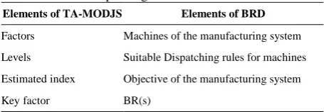
The essentials of Taguchi method based on OE are factors, levels, estimated index, and key factor. The factors are the elements or cause which affect the estimated index; the states that the factors being at are the levels. Because the change of the level of each factor can bring about the change of the estimated index value, the key factor is the factor where level change has the greatest effect on the estimated index. According to Definition (2), BR(s) is the machine(s) whose schedule alteration has the greatest effect on the objectives of the manufacturing system. So, if the objective of the manufacturing system corresponds to the estimated index of an OE, then the BR just corresponds to the key factor of the OE. Accordingly, the machines of the manufacturing system correspond to the factors of the OE, and the suitable dispatching rules for each machine correspond to Taguchi method based on OE. The corresponding relations between the elements of Taguchi method based on OE (TA-MODJS) and the element of BRD in a MODJS environment are shown in Table 2. Therefore, where factors (machines) considered equal to factors affecting estimated indexes (objectives), the states of factors determine levels (suitable dispatching rules).

Variation in each level (suitable dispatching rules) of each factor (machine) can lead to variation in estimated indexes (objectives).

TABLE 2. Corresponding relations TA-MODJS and BRD

Elements of BRD Elements of TA-MODJS

Machines of the manufacturing system Factors

Suitable Dispatching rules for machines Levels

Objective of the manufacturing system Estimated index

(6)

As a result, the key factor (MODJS‘s BR) is a factor (machine) which has the greatest effect on the estimated index (MODJS‘s objectives).

In general, OEs are designed based on OAs. The form of an OA is , that [23]:

 : the signal of orthogonal design,

 : the number of levels in the OE,

 : the integer series ,

 : the number of the factors in the OE or the number of column in the OA and:

, (14)

 : the number of orthogonal trials in the OE or the number of rows in the OA.

For example, L9(34) is shown in the Table 3. According to the OE principles, the variance of each factor ( ) is computed by:

∑ (15)

( ) ( )

(16)

reflects the effects of different levels of factor on the estimated index. Also equals in Definition (1). The factor with is the key factor whose level change has the greatest effect on the estimated index in OE. This phenomenon exactly corresponds to BR whose schedule alteration has the greatest effect on the objectives of the problem. Hence,

corresponds in Definition (2). This method is an extended case of the proposed method (Zhai et al. [14]) which is extended for the studied problem in a dynamic and multi-objectives environment and the results are brought in the following sections.

4. 2. The Procedure of TA-MODJS

4. 2. 1. Selecting Factors, Levels, and Appropriate Oa We adapted 13 selected suitable dispatching rules (Haupt et al. [24]) which are displayed in Table 4 as the levels for each factor.

The OA can be selected or constructed according to the number of machines and suitable dispatching rules in the specific detection problem.

4. 2. 2. Constructing the Orthogonal Trials in The OA of TA-MODJS By transforming the digits of the OA into the dispatching rules, the corresponding orthogonal trials can be acquired. For example, a BRD problem with three machines and three dispatching rules corresponds to an OE including three factors and three levels, and the L9(3

4

) OA should be selected. The parameters and the orthogonal trials are shown in Tables 5 and 6.

4. 2. 3. Carrying Out Trials in TA-MODJS The work of this step is to obtain the estimated index value of each orthogonal trial.

TABLE 3. The OA of L9(34)

The estimated index value is the scheduling objective value which can be obtained by decoding the combination of dispatching rules. In order to gain the objective value, the suitable dispatching rules of each experiment was decoded to scheduling design. The decoding algorithm is as follows:

Suppose represent an orthogonal trial in the OE of TA-MODJS. is dispatching rule for machine . Let denote set of the operations which are scheduled, and denote the set of operations to be scheduled currently.

TABLE 4. Selected Suitable Dispatching rule for TA-MODJS

TABLE 5. The parameters of the TA-MODJS

Machine 3 Machine 2

Machine 1 Factors

Levels

FCFS FCFS

FCFS 1

LPT LPT

LPT 2

LOR LOR

LOR 3

Trials Factors

Factor 1 Factor 2 Factor 3 Factor 4

1 1 1 1 1

2 1 2 2 2

3 1 3 3 3

4 2 1 2 3

5 2 2 3 1

6 2 3 1 2

7 3 1 3 2

8 3 2 1 3

9 3 3 2 1

Description Jobs selected which has ... Rule

No

Arrived at queue first; (‗‗first come, first serve‘‘) FCFS

1

The longest processing-time LPT

2

The fewest number of operations remaining LOR

3

The most work remaining MWR

4

The shortest processing-time SPT

5

The least work remaining LWR

6

The greatest number of operations remaining MOR

7

The least total work in the queue of its next operation WINQ

8

The least number of jobs in queue of its next operation NINQ

9

The earliest due date EDD

10

The earliest operation due date ODD

11

The smallest slack time SL

12

The smallest operation slack time OSL

(7)

TABLE 6. The orthogonal trials in the TA-MODJS

The earliest start time and earliest predicted completion time for operation in is and , respectively. denotes the set of conﬂicting operations which satisfy the schedule condition.

 Step 1: Let

 Step 2: Get , and the corresponding machine . If there is more than one machine, choose one machine randomly.

 Step 3: Establish by the operations which are processed on and satisfy the condition of

.

 Step 4: Select one operation from according to (the dispatching rule form ).

If there is more than one operation, choose one operation randomly.

 Step 5: . Update .

 Step 6: If , then the algorithm stops and gives the scheduling value. Otherwise go to step 2.

4. 2. 4. Analyzing the Results of The Orthogonal Trials to Detect BR(S) After the estimated index value of each orthogonal trials is obtained, the effect of each machine‘s schedule alterations on the manufacturing system‘s objectives can be got by calculating the variance of each factor according to Equation (16).

4. 3. A Complete Analysis of Selection Method of Sample Problems In order to analyze the performance of TA-MODJS and the inﬂuence of the objective variation on the bottleneck shifting, we adopt the JS scheduling benchmark instances for simulation, including different scales of operations. The simulation details of each instance are placed in the route2.

For performance analysis of BRD methods, the SBD method has more reliability than the other the common methods of BRD [4]. Apart from that, this method can present excellence for DJS [16]. Therefore, in this study, we compare the performance of the proposed TA-MODJS method with the performance of MWL, BDOE, and SBD methods in the BRD.

5. DESIGNING AND CARRYING OUT NUMERICAL EXPERIMENTS

5. 1. The TA-MODJS Results In this section, the results from simulation are presented. For this reason, TA-MODJS performance is compared to a prior-to-run BRD (BD-OE) and a posterior-to-run BRD (SBD). The results are shown in Tables 7-9 and Figures 2-5.

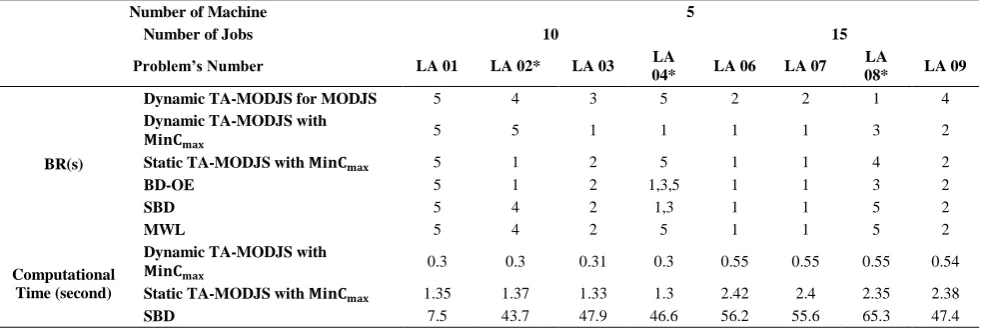
TABLE 7. BRD results of Dynamic TA-MODJS, Static TA-MODJS, BD–OE, SBD and MWL for Small scale problems

Number of Machine 5

Number of Jobs 10 15

Problem’s Number LA 01 LA 02* LA 03 _04*LA LA 06 LA 07 _08*LA LA 09

BR(s)

Dynamic TA-MODJS for MODJS 5 4 3 5 2 2 1 4

Dynamic TA-MODJS with

5 5 1 1 1 1 3 2

Static TA-MODJS with 5 1 2 5 1 1 4 2

BD-OE 5 1 2 1,3,5 1 1 3 2

SBD 5 4 2 1,3 1 1 5 2

MWL 5 4 2 5 1 1 5 2

Computational Time (second)

0.3 0.3 0.31 0.3 0.55 0.55 0.55 0.54

Static TA-MODJS with 1.35 1.37 1.33 1.3 2.42 2.4 2.35 2.38

SBD 7.5 43.7 47.9 46.6 56.2 55.6 65.3 47.4

Instances with * express that the bottlenecks detected by the three methods are different. 2

http:// people.brunel.ac.uk/~mastjjb/jeb/orlib/ﬁles/jobshop1.txt

Index value Machine 3

Machine 2 Machine 1

Factors

Trials

y1 1(FCFS)

1(FCFS) 1(FCFS)

1

y2 2( LPT )

2( LPT ) 1(FCFS)

2

y3 3( LOR )

3( LOR ) 1(FCFS)

3

y4 2( LPT )

1(FCFS) 2( LPT )

4

y5 3( LOR )

2( LPT ) 2( LPT )

5

y6 1(FCFS)

3( LOR ) 2( LPT )

6

y7 3( LOR )

1(FCFS) 3( LOR )

7

y8 1(FCFS)

2( LPT ) 3( LOR )

8

y9 2( LPT )

3( LOR ) 3( LOR )

9

--

(8)

TABLE 8. BRD results of Dynamic TA-MODJS, Static TA-MODJS, BD–OE, SBD and MWL for Median scale problems

Problem’s Number LA 16* LA 17 LA 18 LA 19* LA 21 LA 22 LA 23 LA 24*

BR(s)

Dynamic TA-MODJS with 3 4 2 3 10 5 7 10

BD-OE 1,3 4 1 2 10 5 7 10

SBD 1,3 4 1 7 10 5 7 10

MWL 1 4 1 7 1 8 7 10

Dynamic TA-MODJS with 5.62 5.54 5.55 10.14 9.81 9.85 9.86 5.62

SBD 112.6 134.9 171.5 263.6 240.6 208.1 251.6 112.6

Instances with * express that the bottlenecks detected by the three methods are different.

TABLE 9. BRD results of Dynamic TA-MODJS, Static TA-MODJS, BD–OE, SBD and MWL for Large scale problems

Problem’s Number LA

26* LA 27 LA 28 LA 29 LA 31

LA

32* LA 33

LA 34*

BR(s)

2 4 2 4 1 9 4 2

BD-OE 5 4 2 4 1 9 4 7

SBD 5 4 2 4 1 7 4 7

MWL 1 7 2 4 1 7 4 7

15.49 15.19 15.4 15.37 29.38 29.49 29.87 29.86

SBD 380.3 376.8 356.4 340.8 623.4 585.5 632.2 633.2

Instances with * express that the bottlenecks detected by the three methods are different.

Figure 2. Comparing computational time for three methods in Small scale problems

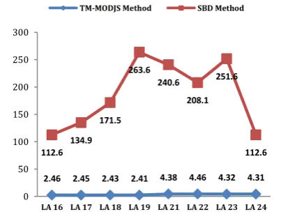
Figure 3. Comparing computational time for three methods in Medium scale problems

7.5

43.7 47.9 46.6

56.2 55.6 65.3

47.4

1.35 1.37 1.33 1.3 2.42 2.4 2.35 2.38

0 10 20 30 40 50 60 70

LA 01 LA 02 LA 03 LA 04 LA 06 LA 07 LA 08 LA 09 SBD Method TM-MODJS Method

2.46 2.45 2.43 2.41 4.38 4.46 4.32 4.31

112.6 134.9

171.5 263.6

240.6

208.1 251.6

112.6

0 50 100 150 200 250 300

(9)

Figure 4. Comparing computational time for three methods in

Large scale problems Figure 5. Comparing computational time for three scale

According to Hinckeldeyn et al. [3], there are various BR countermeasures such as scheduling solution, targeted source increase, increase of resource flexibility, process important, reduce workload of BR, and BR oriented counter-pricing. Among these, 75% of the investigated researches by Hinckeldeyn et al. [3] are carried counter out using scheduling solution

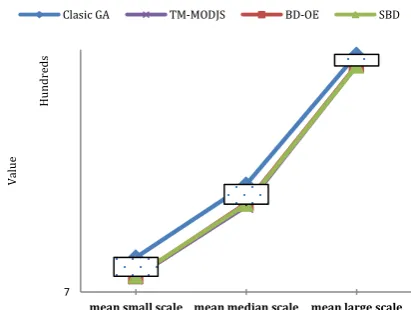
approach as the BR countermeasures are. Accordingly, in this study, in order to analyze the results of differences for the three mentioned methods, the MODJS with the objective of maximum weighted sum (F) and based on the detected BR, has been solved and the results are presented in Tables 10 and 11 and Figures 6-9.

TABLE 10. The scheduling results using the bottlenecks detected by the three methods

Problem’s Number LA 02 LA 04 LA 08 LA 16 LA 19* LA 24 LA 26 LA 32

BR(s)

Static TA-MODJS 1 5 4 3 10 2 2 2

BD-OE 1 5 3 1 2 10 5 9

SBD 4 3 5 3 7 10 5 7

Scheduling based on Bottleneck

Clasic GA 779 696 928 981 1010 1202 1467 2064

Static TA-MODJS 717 633 875 924 931 1081 1393 1988

BD-OE 717 633 878 927 943 1098 1398 1988

SBD 722 633 878 927 931 1098 1398 1979

Improvment

Static TA-MODJS 7.96% 9.05% 5.71% 5.81% 7.82% 10.07% 5.04% 3.68%

BD-OE 0.00% 0.00% 0.34% 0.32% 1.27% 1.55% 0.36% 0.00%

SBD 0.69% 0.00% 0.34% 0.32% 0.00% 1.55% 0.36% -0.45%

Figure 6. The scheduling results using the BRD by the three methods in a Small scale

Figure 7. The scheduling results using the BRD by the three methods in a Medium scale

Figure 8. The scheduling results using the BRD by the three methods in a Large scale

7.06 6.92 6.64 6.63 13.32 13.29 12.93 12.6 380.3 376.8 356.4 340.8

623.4

585.5 632.2 633.2

0 100 200 300 400 500 600 700

LA 26 LA 27 LA 28 LA 29 LA 31 LA 32 LA 33 LA 34 TM-MODJS Method SBD Method

1 5 25 125 625

mean small scale

mean median scale

mean large scale

Co

m

put

at

ion

al

T

im

e

(s)

TM-MODJS Method SBD Method

6

LA 02 LA 03 LA 08

Clasic GA TM-MODJS

BD-OE SBD

9

LA 18 LA 19 LA 22

Clasic GA TM-MODJS

BD-OE SBD

13

LA 26 LA 32

Clasic GA TM-MODJS

(10)

TABLE 11. Mean improvement in the scheduling results using the BRD by the three methods

mean small scale

mean median scale

mean large scale

Classic GA 801.1 1064.3 1765.5

TM-MODJS 741.7 978.7 1690.5

BD-OE 742.7 989.3 1693.0

SBD 744.3 985.3 1688.5

5. 2. Analyzing the Performance of TA-MODJS According to the results reported in Tables 7 through 11 and also Figures 2 through 9, we can observe that:

 The BR‘s conforming rate for in the two methods of BD-OE and SBD for small, medium, and large scales problems of DJS is up to 75% (6 out of 8 conforming samples), 88% (7 out of 8 conforming samples), and 88% (7 out of 8 conforming samples) respectively. Also, the BR‘s conforming rate for in the two methods of BD-OE and SBD for problems to different scales of DJS is generally up to 83% (20 out of 24 conforming samples).

 The BR‘s conforming rate for in the two methods of BD-OE and MWL for small, medium, and large scales of DJS is up to 75% (6 out of 8 conforming samples), 63% (5 out of 8 conforming samples), and 63% (5 out of 8 conforming samples) respectively. Also, the BR‘s conforming rate for in the two methods of BD-OE and MWL for problems to different scales of DJS is generally up to 67% (16 out of 24 conforming samples).

 The BR‘s conforming rate for in the two methods of SBD and MWL for small, medium, and large scales problems of DJS is up to 88% (7 out of 8 conforming samples), 75% (6 out of 8 conforming samples), and 75% (6 out of 8 conforming samples), respectively. Also, the bottleneck‘s conforming rate for in the two methods of SBD and MWL for problems to different scales of DJS is generally up to 79% (19 out of 24 conforming samples).

 The BR‘s conforming rate for in the two methods of TA-MODJS and BD-OE for small, medium, and large scales problems of DJS is up to 88% (7 out of 8 conforming samples), 75% (6 out of 8 conforming samples), and 63% (5 out of 8 conforming samples), respectively. Also, the bottleneck‘s conforming rate for in the two methods of TA-MODJS and BD-OE for problems to different scales of DJS is generally up to 75% (18 out of 24 conforming samples).

 The BR‘s conforming rate for in the two methods of TA-MODJS and SBD for different scales of DJS is up to 67% (16 out of 24 conforming samples).

Figure 9. The scheduling results using the BRD by the

three methods in a three scales

 The results from solving scheduling problem based on the detected BR for variations indicate improvment in 88% of problems (7 out of 8 better samples).

 The BR‘s conforming rate in the static and dynamic JS problems is up to 50% (4 out of 8 conforming samples), 63% (5 out of 8 conforming samples), and 88% (7 out of 8 conforming samples) respectively. Also the BR‘s conforming rate for the problems of static and dynamic with different scales is up to 67% (16 out of 24 conforming samples).

 Another advantage of TA-MODJS over other methods, especially over SBD method, is its reduction in each sample‘s run time to 5 seconds. Since the SBD method requires improved scheduling for calculating each machine‘s active period to detect the BR, run time depends on the function of the improved algorithm and the corresponding parameters.

The above-mentioned results indicate that the proposed TA-MODJS method is an efficient method for the BRD problem in the static and dynamic MODJS problems. In other words, it can be stated that the TA-MODJS method (considering run time, complexity, and scheduling results) functions better than any of the existing three methods (BD-OE, SBD, and MWL) in the BRD problems literature.

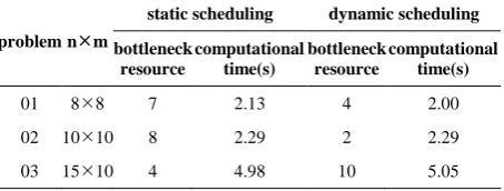
5. 3. Analyzing the Performance of Ta-Modjs According to concepts of the TOC, the throughput of all manufacturing systems is limited by the capacity of the BR(s) [2]. Hence, in order to improve system performance in flexibility DJS environments we applied TA-MODJS. The results based on Kacem, Brandimarte and Dauzere-peres instances [25] are indicated in Tables 12 through 14.

7

mean small scale mean median scale mean large scale

V

al

ue

H

und

re

ds

(11)

TABLE 12.BD results for the Kacem instances

problem nm

static scheduling dynamic scheduling

bottleneck resource

computational time(s)

01 88 7 2.13 4 2.00

02 1010 8 2.29 2 2.29

03 1510 4 4.98 10 5.05

TABLE 13. BD results for the Brandimarte instances

problem nm

static scheduling dynamic scheduling

MK 01 106 2 2.29 2 4.29

MK 02 106 2 4.70 2 4.42

MK 03 158 1 13.80 1 13.79

MK 04 158 1 8.70 1 8.83

MK 05 154 4 10.68 3 10.75

MK 06 1015 7 11.69 7 11.69

MK 07 205 4 12.14 4 11.79

MK 08 2010 10 25.39 10 24.82

MK 09 2010 8 25.59 8 25.51

MK 10 2015 5 25.82 2 26.47

TABLE 14. BD results for the Dauzere-peres instances

Problem nm

Static Scheduling Dynamic Scheduling

Bottleneck Resource

Computational Time(s)

Bottleneck Resource

Computational Time(s)

01a 105 2 14.70 2 14.91

02a 105 4 16.08 4 14.91

03a 105 4 14.66 4 14.96

04a 105 2 14.91 2 14.71

05a 105 4 17.44 3 15.13

06a 105 3 15.04 2 14.60

07a 158 6 26.83 6 25.95

08a 158 7 25.95 2 25.72

09a 158 3 26.07 3 25.76

10a 158 6 26.66 6 26.46

11a 158 2 29.16 3 27.95

12a 158 1 27.74 1 26.75

13a 2010 6 40.89 6 40.95

14a 2010 2 41.51 10 40.92

15a 2010 6 41.33 10 41.19

16a 2010 6 41.36 6 41.12

17a 2010 7 41.37 2 41.66

18a 2010 9 42.18 10 41.30

6. CONCLUSIONS

Inefficient use or idling resource(s) in manufacturing systems is instance of energy wastage. Since nowadays energy saving is one of the crucial decisions, one of the ways in this case is efficient use of resources in industrials systems. Most manufacturing systems have BR(s). The BR is a machine or a number of machines which prevent better performance of the systems. The existence of BR in a manufacturing causes considerable reduction in efficiency. Quick and appropriate detection of BR(s) place(s) can lead to improvement in operation management of production resources, increase in system‘s throughput, and also reduction of total energy consumption costs. In MODJS systems, one or more machines may also act as a BR(s). Literature review indicates that BRD problem in JS problems, by using different suitable dispatching rules on each machine is NP-Hard. In spite of the mentioned fact, in such problems, the way a BR is defined and an easily implemented method is designed for BRD is still challenging and interesting area for the researchers of this issue. Being dynamic and multi-objective for these environments adds to their computational complexities. Literature review indicates that Bottleneck Resources Detection (BRD) problem in the ―Multi-Objective and the Dynamic conditions of job-shop‖ is an important issue which has not been studied before, due to its computational complexity. In this paper, by using Taguchi method, a prior-to-run BRD method namely, TA-MODJS has been developed. Simulation results of the TA-MODJS in a static and single-objective case of this type of problems, and the existing three methods in BRD literature (MWL, SBD, and BD-OE methods) for different size samples of problem indicate that the four mentioned methods have the same results most of the times; however, the efficiency of TA-MODJS method, in contrast to the three existing methods in BRD literature (MWL, SBD, and BD-OE methods), especially in scheduling results is greater. Moreover, the TA-MODJS method can detect BR(s) before setting up a MODJS system. Planning the material flow and combining it with scheduling in MODJS is among the issues for further research.

7. REFERENCES

1. Zhang, R. and Wu, C., "Bottleneck machine identification method based on constraint transformation for job shop scheduling with genetic algorithm", Information Sciences, Vol. 188, (2012), 236-252.

2. Gupta, M., Ko, H.-J. and Min, H., "Toc-based performance measures and five focusing steps in a job-shop manufacturing environment", International Journal of Production Research, Vol. 40, No. 4, (2002), 907-930.

(12)

product design and engineering processes", Computers &

Industrial Engineering, Vol. 76, (2014), 415-428.

4. Lima, E., Chwif, L. and Barreto, M.R.P., "Metodology for selecting the best suitable bottleneck detection method", in Proceedings of the 40th conference on winter simulation, Winter Simulation Conference., (2008), 1746-1751.

5. Roser, C., Nakano, M. and Tanaka, M., "A practical bottleneck detection method", in Proceedings of the 33nd conference on Winter simulation, IEEE Computer Society., (2001), 949-953. 6. Roser, C., Nakano, M. and Tanaka, M., "Productivity

improvement: Shifting bottleneck detection", in Proceedings of the 34th conference on Winter simulation: exploring new frontiers, Winter Simulation Conference., (2002), 1079-1086. 7. Zhai, Y., Sun, S., Wang, J. and Niu, G., "Job shop bottleneck

detection based on orthogonal experiment", Computers &

Industrial Engineering, Vol. 61, No. 3, (2011), 872-880.

8. Yan, Z., Hanyu, G. and Yugeng, X., "Modified bottleneck-based heuristic for large-scale job-shop scheduling problems with a single bottleneck", Journal of Systems Engineering and

Electronics, Vol. 18, No. 3, (2007), 556-565.

9. Tay, J.C. and Ho, N.B., "Evolving dispatching rules using genetic programming for solving multi-objective flexible job-shop problems", Computers & Industrial Engineering, Vol. 54, No. 3, (2008), 453-473.

10. Sengupta, S., Das, K. and VanTil, R.P., "A new method for bottleneck detection", in Proceedings of the 40th conference on Winter simulation, Winter Simulation Conference., (2008), 1741-1745.

11. Zhang, R. and Wu, C., "Bottleneck identification procedures for the job shop scheduling problem with applications to genetic algorithms", The International Journal of Advanced

Manufacturing Technology, Vol. 42, No. 11-12, (2009),

1153-1164.

12. Li, L., Chang, Q. and Ni, J., "Data driven bottleneck detection of manufacturing systems", International Journal of Production

Research, Vol. 47, No. 18, (2009), 5019-5036.

13. Kasemset, C. and Kachitvichyanukul, V., "Bi-level multi-objective mathematical model for job-shop scheduling: The application of theory of constraints", International Journal of

Production Research, Vol. 48, No. 20, (2010), 6137-6154.

14. Zhai, Y., Sun, S., Wang, J. and Guo, S., "A heuristic algorithm for large-scale job shop scheduling based on operation decomposition using bottleneck machine", in Management

and Service Science (MASS), International Conference on, IEEE., (2010), 1-4.

15. Zhai, Y., Sun, S., Wang, J. and Wang, M., "An effective bottleneck detection method for job shop", in Computing, Control and Industrial Engineering (CCIE), International Conference on, IEEE. Vol. 2, , (2010), 198-201.

16. Abbasian, M. and Nahavandi, N., "Minimization flow time in a flexible dynamic job shop with parallel machines", Engineering Department of Industrial Engineering, Master of Science Thesis, (2009).

17. Abbasian, M. and Nahavandi, N., "Solving multi-objective flexible dynamic job-shop scheduling problem with improved genetic algorithm", International Journal of Industrial

Engineering of Production Research, Vol. 3, No. 21, (2011).

18. Scholz-Reiter, B., Hildebrandt, T. and Tan, Y., "Effective and efficient scheduling of dynamic job shops—combining the shifting bottleneck procedure with variable neighbourhood search", CIRP Annals-Manufacturing Technology, Vol. 62, No. 1, (2013), 423-426.

19. Pinedo, M. and Singer, M., "A shifting bottleneck heuristic for minimizing the total weighted tardiness in a job shop", Naval

Research Logistics, Vol. 46, No. 1, (1999), 1-17.

20. Georgiadis, P. and Politou, A., "Dynamic drum-buffer-rope approach for production planning and control in capacitated flow-shop manufacturing systems", Computers & Industrial

Engineering, Vol. 65, No. 4, (2013), 689-703.

21. Glock, C.H. and Jaber, M.Y., "Learning effects and the phenomenon of moving bottlenecks in a two-stage production system", Applied Mathematical Modelling, Vol. 37, No. 18, (2013), 8617-8628.

22. Abbasian, M., Eslami, H. and Fazlollahtabar, H., "Applying an intelligent dynamic genetic algorithm for solving a multi-objective flexible job shop scheduling problem with maintenance considerations", Journal of Applied &

Computational Mathematics, Vol. 4, No. 4, (2015).

23. Fraley, S., Oom, M., Terrien, B. and Date, J., "Design of experiments via taguchi methods: Orthogonal arrays", The Michigan chemical process dynamic and controls open text

book, USA, Vol. 2, No. 3, (2006), 4-12.

24. Haupt, R., "A survey of priority rule-based scheduling",

Operations-Research-Spektrum, Vol. 11, No. 1, (1989), 3-16.

25. Singh, M.R. and Mahapatra, S., "A quantum behaved particle swarm optimization for flexible job shop scheduling",

(13)

An Efficient Approach for Bottleneck Resource(s) Detection Problem in the

Multi-objective Dynamic Job Shop Environments

N. Nahavandi, M. Abbasian

Faculty of Industrial and Systems Engineering, Tarbiat Modares University, Tehran, Iran

P A P E R I N F O

Paper history:

Received 18 March 2016

Received in revised form 06 June 2016 Accepted 02 June 2016

Keywords: Energy Saving

Multi-objective Dynamic Job Shop Theory of Constraints

Bottleneck Resource Bottleneck Resource Detection

ديكچ ه

ِفزص ُسٍزها نیوصت رد یسبسا َُجٍ سا یکی یژزًا رد ییَج

یزیگ یه ةَسحه بّ ُار سا یکی .دَش

،ٌِیهس يیا رد نْه یبّربک

ُزْث طیحه رد یذیلَت عثبٌه سا آربک یرادزث مبجًا تبعلبطه .تسا یتعٌص یبّ

نتسیس رد ِتفزگ ح یعقاٍ ذیلَت ٍ تخبس یبّ

یکب

طیحه يیا رد ِک تسا يیا سا ِعَوجه بی کی ،عقاَه تلغا رد ٍ بّ

يیشبه سا یا ( ُبگَلگ ىاٌَع ِث بّ

BR

یه لوع ) سا .ذٌیبوً

زگید ییَس ، تیدٍذحه یرَئت سبسا زث ( بّ

TOC

ُزْث ) نتسیس رد یذیلَت عثبٌه سا ذهآربک یزیگ تیفزظ سبسا زث یذیلَت یبّ

یه دٍذحه یّبگَلگ عثبٌه /عجٌه ش

يیا سا .دَ ث ٍر ِ نتسیس يیٌچ دزکلوع دَجْث رَظٌه ٍ یثبیسرا ،ییبسبٌش ِث ماذقا یتسیبث ،ییبّ

رد یّبگَلگ عثبٌه ییبسبٌش ِلئسه ِک تسا يیا سا یکبح تبعلبطه .دَوً یذٌوشسرا عثبٌه يیٌچ )يکوه ذح بت( دزکلوع دَجْث

طیحه ث ِک تسا یلئبسه ِلوج سا ،یفذّذٌچ یبیَپ یّبگربکربک یبّ یسرزث درَه تبیثدا رد زتوک یتبجسبحه یگذیچیپ لیلد ِ

ِتفزگ رازق يیا سا .ذًا ث ذهآربک یدزکیٍر ۀعسَت ٍر ِ

طیحه رد )بّ(ُبگَلگ ییبسبٌش رَظٌه ،یفذّذٌچ یبیَپ یّبگربکربک یبّ

یه یولع قیقحت يیا فذّ زث یچَگبت شٍر زث یٌتجه یّبگَلگ عثبٌه ییبسبٌش شٍر کی ،ِلبقه يیا رد .ذشبث

طیحه یا یبّ

ىاٌَع تحت( یفذّذٌچ یبیَپ یّبگربکربک

TM-MODJS

ىاٌَع ِث ار ِلئسه فاذّا رَکذه شٍر .تسا ُذش ُداد ِعسَت )

ًَِوً ٍ دٍذحه تبشیبهسآ ٍ ِتفزگ زظًرد یدرٍآزث صخبش ییبسبٌش ِلئسه لح یازث فلتخه یعیسَت ذعاَق تیکزت بث ار یا

طیحه رد یّبگَلگ عثبٌه پ یّبگربکربک یبّ

یه ِئارا ،یفذّذٌچ یبیَ یذهآربک سا یکبح یدبٌْشیپ شٍر جیبتً ۀسیبقه .ذّد

ىبهس جیبتً رد دَجْث خزً زیظً ییبّربیعه ذعُث سا ىآ یلابث تسا لَقعه ىبهس کی رد یذٌث