Using Multiple Calibration Sets to
Im-prove the Quantitative Accuracy of
Partial Least Squares (PLS) Regression
on Open-Path Fourier Transform
In-frared (OP/FT-IR) Spectra of Ammonia
over Wide Concentration Ranges
LIMIN SHAO,* BIANXIA LIU, PETER
R. GRIFFITHS, and APRIL B.
LEYTEM
Department of Chemistry, University of Science and Technology of China, Hefei, Anhui 230026, P.R. China (L.S., B.L.); Department of Chemistry, University of Idaho, Moscow, Idaho 83844-2343 (P.R.G.); and United States Department of Agriculture, Agricultural Research Service, Northwest Irrigation and Soils Research Laboratory, Kimberly, Idaho 83341
The use of multiple calibration sets in partial least squares (PLS) regression was proposed to improve the quantitative determination of NH3over wide concentration ranges from open-path Fourier transform
infrared (OP/FT-IR) spectra. The spectra were measured near animal farms, where the path-integrated concentration of NH3can fluctuate from
nearly zero to as high as approximately 1000 ppm-m. PLS regression with a single calibration set did not cover such a large concentration range effectively, and the quantitative accuracy was degraded due to the nonlinear relationship between concentration and absorbance for spectra measured at low resolution (1 cm1and poorer.) In PLS regression with
multiple calibration sets, each calibration set covers a part of the entire concentration range, which significantly decreases the serious nonlinearity problem in PLS regression occurring when only a single calibration set is used. The relative error was reduced from approximately 6% to below 2%, and the best results were obtained with four calibration sets, each covering one quarter of the entire concentration range. It was also found that it was possible to build the multiple calibration sets easily and efficiently without extra measurements.
Index Headings:Open-path Fourier transform infrared spectrometry; OP/ FT-IR spectrometry; Partial least squares; PLS regression; Quantitative accuracy; Calibration.
INTRODUCTION
Open-path Fourier transform infrared (OP/FT-IR) spectrom-etry is an effective technique to measure the concentration of greenhouse gases and other molecules in the atmosphere.1 Atmospheric monitoring of the gaseous emissions from various sources, such as industrial plants, agricultural operations, engines of motor vehicles or aircraft, etc., has also been reported by this technique.2–4The instrumentation for OP/FT-IR spectrometry is rugged and relatively easy to operate in the field.5–9 However, data analysis is rather difficult because the spectra are complicated by the dominant and omnipresent absorption bands of atmospheric water vapor and CO2, the
concentration and temperature of which change constantly, and by the deviations from Beer’s law for narrow lines in the vibration-rotation spectra of small molecules measured at low or medium resolution.10 To reduce the effects of these uncontrollable factors, we have shown that the application of partial least squares (PLS) regression is preferable to other chemometric methods.11,12 However, when the concentration of an analyte varies over a very wide range, as it does around animal farms, for example, even PLS regression leaves room for improvement.
In PLS regression, the calibration spectra must be measured under conditions for which all sources of variance in the spectra to be analyzed are encompassed even though not all the variables need be quantified. If the analyte occurs at very high concentration (such as NH3in the atmosphere around animal farms), the range of path-integrated concentrations for the calibration set should exceed the highest value that will be encountered in the field. Such a large concentration range may result in significant nonlinearity between measured absorbance and concentration. Although the effect of nonlinearity can in principle be managed by including more factors in the PLS model, the number of calibration spectra must then be increased, which can present a problem in practice for OP/ FT-IR measurements.
Several attempts to ameliorate the effect of nonlinearity over a wide concentration range have been reported. In a study of classical least squares (CLS) calibration for methane, Ropertz separated spectra taken over a large concentration range (20 to 10000 ppm-m) into two parts and built a linear and a second-order model, with the latter giving a lower root mean square error of prediction (RMSEP).13Bak and Larsen used linearized CO spectra as input to the PLS regression; in this case the calibration model was found to have good predictive ability throughout the entire concentration range from 15 to 32 640 ppm-m.14 Alcala et al. investigated the effect of the concentration range in the calibration model on the prediction of low concentrations of pharmaceutical compounds.15 Even though the bands they measured in the spectra were broader than those in most OP/FT-IR measurements, they concluded that the selection of wide concentration ranges was not recommended for the determination of analytes at minor levels, even when the concentration of the analyte is within the range of the model.
In our investigations of the atmosphere around animal farms, we found that the path-integrated concentration of NH3 can fluctuate from nearly zero to as high as approximately 1000 ppm-m.16 For the highest path-integrated concentrations, the true peak absorbance (i.e., the peak absorbance measured at infinitely high resolution) exceeds 1.0 and linear Beer’s law behavior is not observed when the spectrum is measured with a resolution parameter greater than unity. Highly nonlinear behavior would be expected with boxcar truncation or triangular apodization,17 but even with the Norton–Beer apodization functions, some nonlinearity is predicted.18 In order to be able to process OP/FT-IR spectra measured adjacent to a dairy production facility19 when the NH
3 concentration covers a wide range, we used a calibration set for the PLS regression of NH3for which the NH3concentration ranged from 0 to 1400 ppm-m. Use of a calibration set with this wide range of concentration led to good prediction perfor-mance for spectra of either low, medium, or high concentration, but not throughout the entire range. Better results were
Received 16 February 2011; accepted 22 April 2011.
* Author to whom correspondence should be sent. E-mail: limin.shao@ gmail.com.
obtained when more than one calibration set was used, with each set covering a part of the entire concentration range.
In this paper, we report the result of dividing the data set containing a large concentration range into smaller sets and building a calibration set for each smaller range. The OP/FT-IR spectrum to be analyzed is first subjected to a PLS regression with a single calibration set that covers the entire concentration range and the approximate concentration of NH3is obtained. Then, one of the multiple calibration sets is selected so that its concentration range includes the approximate concentration and another PLS regression is performed on the same spectrum to yield a‘‘refined’’concentration. Results indicated significant improvement in the accuracy of the predicted concentrations of NH3. It was also found that it was possible to build the multiple calibration sets easily and efficiently from quantitatively accurate reference spectra without actual experiments.
MEASUREMENT AND DATA PROCESSING
Experimental. OP/FT-IR spectra were measured in a
cooperative project for monitoring gaseous emissions around animal farms in southern Idaho with the Northwest Irrigation and Soil Research Laboratory of the United States Department of Agriculture’s Agricultural Research Service. The OP/FT-IR spectrometer was manufactured by MDA Corp. (Atlanta, GA) and incorporated a Bomem Michelson 100 interferometer, a 31.5 cm telescope, a cube-corner array retro-reflector, and a Sterling engine-cooled mercury cadmium telluride (MCT) detector. Interferograms were measured with a maximum optical path difference of 1 cm (nominal resolution of 1 cm1), then corrected for the nonlinear response of the MCT detector.20 All OP/FT-IR spectra were computed from the interferograms with a zero-filling factor of 8 and medium Norton–Beer (MNB) apodization.
Spectral data in the region from 1250 to 750 cm1were used for the PLS regression to predict the concentration of NH3. All manipulation of spectra and data processing were done using MATLAB 7.0.1 (The Math-Works Inc., Natick, MA) on the Windows Vista operating system.
Calibration and Validation Sets.The calibration set in PLS
regression was composed of 54 spectra with different path-integrated concentrations of NH3. For measurements made in open air, it is impossible to control the release of NH3such that the concentration along the entire path length (which is usually between 100 and 200 m) is uniform, which is why path-integrated concentrations (in ppm-m) are measured rather than simply concentration. These spectra were synthesized by first acquiring 54 single-beam background OP/FT-IR spectra in pristine air over a period of several months. These spectra were measured with a variety of path lengths (from 50 to 500 m), temperatures (108C,T, 358C), and relative humidities to ensure that all sources of variance of the background were encompassed. Each spectrum was ratioed against a single-beam background spectrum measured with the retro-reflector within 1 m of the telescope and converted to absorbance. Then, 54 reference spectra of NH3 with different concentrations were prepared in the way described by us previously.21,22 A high-resolution (0.125 cm1) reference absorbance spectrum of ammonia was first multiplied by a known, randomly selected scaling factor and then converted to transmittance. The fast Fourier transform (FFT) of the transmittance spectrum was then calculated and the resulting array was truncated to an optical path difference of 1 cm and apodized with the Norton–
Beer medium function to make the resolution and instrument line-shape function equal to that of the background spectrum. The inverse FFT of this array was then calculated to give the transmittance spectrum under the same conditions as the background spectrum and converted to absorbance. Each ammonia spectrum calculated in this way was added to an absorbance spectrum of pristine air. These composite spectra reflect the full range of conditions under which the OP/FT-IR spectra were measured in the field.
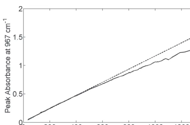
Several sets of OP/FT-IR spectra were acquired in the field under the same conditions as the spectra in the calibration set, but with different concentrations of NH3. Because it is impossible to control the release of NH3in open air, we chose a number of OP/FT-IR spectra that had been measured around animal farms with different levels of NH3 and calculated the corresponding concentrations. The concentration could not be calculated by directly applying Beer’s law, because the high absorbance of NH3results in significant nonlinearity between absorbance and concentration. Instead, we used an iterative procedure to estimate the concentrations accurately. This procedure is followed because high-resolution spectra obey Beer’s law over a wide concentration range, but this is not the case for low-resolution spectra.21The high-resolution reference spectrum of ammonia (in absorbance) was first multiplied by a tentative scaling factor and deresolved using the same procedure used for the calibration spectra. The deresolved spectrum was subtracted from the measured validation spectrum to give a residual spectrum. The above procedure was repeated with the scaling factor varied iteratively until the residual spectrum showed no absorption line due to NH3 between 970 cm1and 960 cm1(in which the strongest line in the ammonia spectrum is located). The concentration of NH3 was determined from the final scaling factor. With this procedure, a validation set of 63 spectra that were completely independent of the calibration spectra was obtained that covered a concentration of NH3from 33 to 1400 ppm-m. We checked the relationship between the concentrations and the peak absorbance at 967 cm1, at which the most intense absorption of NH3occurs, and found significant deviation from Beer’s law, as shown in Fig. 1. It is also noteworthy that in the case of very high absorbance of NH3, the IR beam reaching the detector near the wavenumber of maximum absorption is so weak that the noise level near the peak of the absorption band can be very high and estimates of the concentration of NH3 may be affected.
RESULTS AND DISCUSSION
In PLS regression with a single calibration set (subsequently referred to as SCS) the concentration range of NH3 was set from 0 to 1400 ppm-m. For PLS with multiple calibration sets the large concentration range was divided into N segments evenly, and for each segment an independent calibration set was built. Those N calibration sets compose the multiple calibration sets (subsequently referred to as MCS-N). For MCS-2, for example, there are two calibration sets, one covering the concentration range from 0 to 700 ppm-m, and the other covering 700 to 1400 ppm-m. For the results described in this paper, we investigated the PLS regressions with MCS-2 through MCS-12. So for each of the 63 validation spectra, there are twelve predictions for the concentration of NH3.
Partial Least Squares Regressions with SCS and
regressions with different number of calibration sets, the mean absolute percentage error (MAPE) was calculated as shown in Eq. 1:
MAPE¼1 n
Xn
i¼1
piti
ti
3100 ð1Þ
where nis the number of validation samples;piandtidenote the two calculated concentrations of NH3 from the ith validation sample by PLS and the iterative procedure described above, respectively.
The MAPE values were plotted against the number of multiple calibration sets, N, in Fig. 2. It can be seen that the PLS regression with SCS led to a mean absolute percentage error of about 6%. However, the error drops significantly to about 2%with only two calibration sets (MCS-2), as shown in the plot. The relative error continues to decrease with the number of calibration sets, and after MCS-4, tends to be stable, at about 1.5%.
The results revealed a clear improvement when using multiple calibration sets in the PLS regression because this strategy effectively reduces the effect of nonlinearity between measured absorbance and concentration. The single calibration set covers the large concentration range from 0 to 1400 ppm-m, and the 54 spectra in the SCS might be inadequate to reduce the nonlinearity considerably. But in MCS-N, each calibration set covers only a small range with the length being 1400/N ppm-m. Nonlinearity over each small concentration range is much less serious than over the large range that was covered by the SCS, so the quantitative accuracy is improved.
We found that the number of factors in the PLS regression with multiple calibration sets varies. For example, with MCS-6, for the six PLS models that cover the concentration ranges of 0–233, 234–467, 468–700, 701–933, 934-1167, and 1168– 1400 ppm-m, the numbers of factors were found to be 10, 10, 7, 6, 5, and 4, respectively. The reason for the observed variation is that when the concentration of NH3 in the calibration set is low, besides the spectral information due to NH3, absorption of water vapor and the effect of the non-zero
baseline make significant contributions to the PLS model, which results in the need for extra factors. When the concentration of NH3 in the calibration set was high, these other factors became less significant, and the absorption lines of NH3account for the major source of variance for the PLS model, so fewer factors are needed.
The downside of PLS regression with multiple calibration sets is computational complexity. More than one PLS model needs be built independently, and for each spectrum, two PLS regressions are carried out to yield the concentration. However, this procedure has been automated and the regression for each short range is short enough that the additional computational complexity does not present a problem.
Optimized Partial Least Squares Regression with
Multiple Calibration Sets. As noted above, to select the
optimal MCS model with respect to the validation set, we used the criterion of mean absolute percentage error (MAPE). Among the twelve PLS regressions, the minimum value of MAPE was reached at MCS-7; however, MCS-4 and MCS-8 also gave very low MAPE values, as shown in Fig. 2. For a rigorous comparison, we inspected the results of all 63 validation spectra. Figure 3 shows the relative errors of the concentrations predicted by the PLS regressions with MCS-1, MCS-2, MCS-4, MCS-7, and MCS-8.
Figure 3 also shows details about the results of the PLS regressions with SCS and MCS-N. PLS regression with SCS performed well in the range from 200 to 600 ppm-m, where the measured absorbance is approximately proportional to concen-tration, but the errors increased when the concentration of NH3 is less than 200 ppm-m (presumably because the signal-to-noise ratio is not high enough) or greater than 700 ppm-m (where the measured absorbance of the stronger NH3lines is no longer proportional to concentration). As expected from Fig. 3, the results for the PLS regression with MCS-2 were greatly improved over MCS-1 when NH3 was present at high concentration, which helped explain the significant drop of MAPE from MCS-1 to MCS-2 in Fig. 2.
For further comparison, we performed pairedt-tests at 95%
confidence to the concentrations predicted by different PLS
regressions. In this case, the critical valuet0.05,62is 2.00. Thet value between MCS-2 and MCS-3 was calculated to be 1.25, so there is no statistically significant difference between the concentrations predicted by PLS with the two models. However, thet value calculated between MCS-2 and MCS-4, or MCS-3 and MCS-4, is greater than the critical value. Therefore, with a lower MAPE value, MCS-4 is a better model than 2 or 3. The lowest MAPE value is with MCS-7, 1.32, only slightly lower than that of MCS-4, 1.36. The pairedt-test between MCS-4 and MCS-7 reported atvalue of 0.98, smaller than the critical value. Therefore, there is no statistically significant difference between the concentrations predicted by the PLS regressions with MCS-4 and MCS-7. In other words, the PLS regression with MCS-7 is not statistically better than that with MCS-4, even though the MAPE value is slightly smaller. In conclusion, the optimal model can be
MCS-4 or MCS-7. If the computational complexity should be taken into consideration, MCS-4 is the better choice.
CONCLUSION
It was found that PLS regression with multiple calibration sets is more flexible and accurate than using a single calibration set to process the spectra measured around animal farms, where the concentration of NH3varies significantly from nearly zero to approximately 1000 ppm-m. The relative error was reduced from approximately 6%to below 2%, and the best results were obtained with four calibration sets.
ACKNOWLEDGMENTS
This work was funded by contract 58-5368-0-089F with the USDA/NWISL, Agricultural Research Service, Northwest Irrigation and Soils Research Laboratory, Kimberly, Idaho, and by the National Natural Science Foundation FIG. 2. Mean absolute percentage error of PLS regression with different MCS-N.
in China (Grant No. 20705032). This work was also partly funded by the Chinese Universities Scientific Fund.
1. G. M. Russwurm and J. W. Childers, ‘‘Open-path Fourier transform infrared spectroscopy’’, inHandbook of Vibrational Spectroscopy,J. M. Chalmers and P. R. Griffiths, Eds. (Wiley, New York, 2002), vol. 2. 2. A. R. Newman, Anal. Chem.69,43 (1997).
3. W. T. Walter, Proc. SPIE Int. Soc. Opt. Eng.5270,144 (2004). 4. Z. Bacsik, J. Mink, and G. Keresztury, Appl. Spectrosc. Rev. 40,327
(2005).
5. J. W. Childers, E. L. Thompson, D. B. Harris, D. A. Kirchgessner, M. Clayton, D. F. Natschke, and W. J. Phillips, Atmos. Environ.35,1923 (2001). 6. B. Eklund, Atmos. Environ.33,1065 (1999).
7. D. W. T. Griffith, R. Leuning, O. T. Denmead, and I. M. Jamie, Atmos. Environ.36,1833 (2002).
8. S. Briz, J. Barrancos, D. Nolasco, G. Melia´n, E. Padro´n, and N. Pe´rez, Proc. SPIE Int. Soc. Opt. Eng.7475,747510-1 (2009).
9. K. Scha¨fer, C. Jahn, M. Wiwiorra, A. Schleichardt, S. Emeis, A. Raabe, J. Bo¨ttcher, N. D. Landmeyer, C. Bonecke, M. Deurer, C. von der Heide, and D. Weymann, Proc. SPIE Int. Soc. Opt. Eng.7475,747511-1 (2009).
10. P. R. Griffiths and J. A. de Haseth, Fourier Transform Infrared Spectrometry(Wiley-Interscience, Hoboken, NJ, 2007), 2nd ed., p. 177. 11. B. K. Hart and P. R. Griffiths, Environ. Sci. Technol.34,1346 (2000). 12. L. Shao, P. R. Griffiths, and A. B. Leytem, Anal. Chem.82,8027 (2010). 13. A. Ropertz, T. Lamp, M. Douard, K. Weber, A. Gaertner, C. Elbers, and R.
Nitz, Proc. SPIE Int. Soc. Opt. Eng.3107,137 (1997). 14. J. Bak and A. Larsen, Appl. Spectrosc.49,437 (1995).
15. M. Alcala`, J. Leo´n, J. Ropero, M. Blanco, and R. J. Roma˜nach, J. Pharm. Sci.97,5318 (2008).
16. D. L. Bjorneberg, A. B. Leytem, D. T. Westermann, P. R. Griffiths, L. Shao, and M. J. Pollard, Trans. ASABE52,1749 (2009).
17. R. J. Anderson and P. R. Griffiths, Anal. Chem.47,2339 (1975). 18. C. Zhu and P. R. Griffiths, Appl. Spectrosc.52,1403 (1998).
19. A. B. Leytem, R. S. Dungan, D. L. Bjorneberg, and A. C. Koehn, ‘‘Emissions of Ammonia, Methane, Carbon Dioxide and Nitrous Oxide from Dairy Cattle Housing and Manure Management Systems’’, J. Environ. Qual. (2010), paper in press.
20. L. Shao and P. R. Griffiths, Anal. Chem.80,5219 (2008).
21. L. Shao, P. R. Griffiths, P. M. Chu, and T. W. Vetter, Appl. Spectrosc.60, 255 (2006).